In the previous two posts (see This and This Post), we learned about important topics regarding networking and compute services. Now, we will continue by looking at another fundamental offering from GCP – storage. Every application needs to store data, but not all data is the same. Data can be structured, unstructured, relational, or transactional, and GCP offers services to meet these requirements. Your application may even need to use multiple storage services to achieve your needs.
In this article, we will look at the different types of storage offered by Google and explain what should be considered before selecting a particular service. Google provides numerous storage options and covering all of these in a single post may make the facts difficult for you to digest. Therefore, we have divided this blog into two parts.
In this part, we will consider which storage option we should choose and look into the following topics:
- Choosing the right storage option
- Understanding Cloud Storage
- Understanding Cloud Firestore
- Understanding Cloud SQL
Although BigQuery can be considered a storage option, we will look at that product in This Post, Analyzing Big Data Options.
Let's start this article by looking at when we should select a specific storage service. After that, we will look at each service individually while concentrating on exam topics.
Choosing the right storage option
As we mentioned at the beginning of this post, various storage services are offered by Google. You must understand what the correct storage to use is for your requirements. Google provides a nice flow chart that we can walk through. It is easy to follow and shows how requirements will dictate which storage option to select. Take some time to look at the following decision tree. This diagram works through some key questions to make sure that the storage service we select will fulfill our requirements:
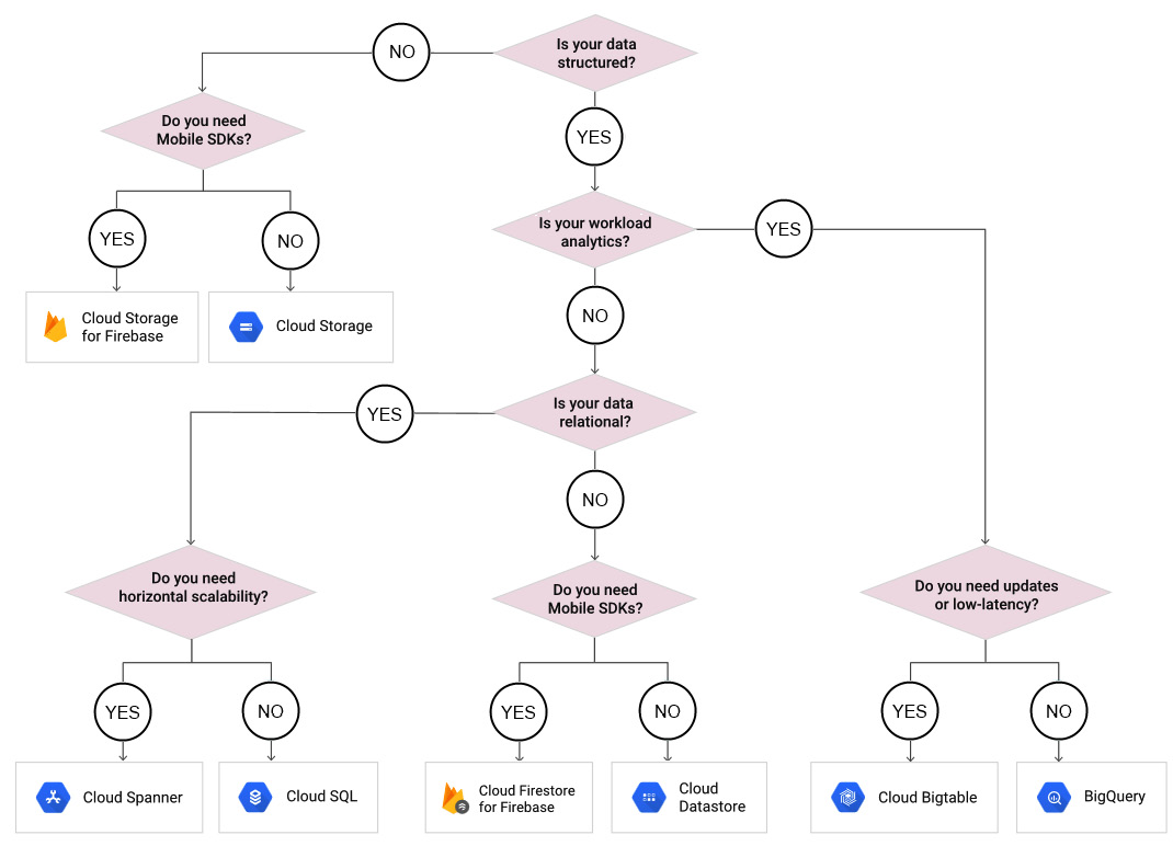
Figure 11.1 – Storage options
With the preceding diagram in mind, let's walk through an example:
- First, we need to understand whether our data will be structured. Different services will be recommended, depending on this answer.
- If our data is structured, then we should check whether our workload is for analytics.
- If our data is not for analytics, then we should check whether our data is relational.
- If our data is relational, then we need to know whether we require horizontal scaling.
- If we do, then we should select Cloud Spanner. If not, we should select Cloud SQL.
As shown in the preceding diagram, there are various outcomes, depending on our requirements. There are a lot of storage services offered by GCP, but if we follow this flow chart, we should be able to choose the best option.
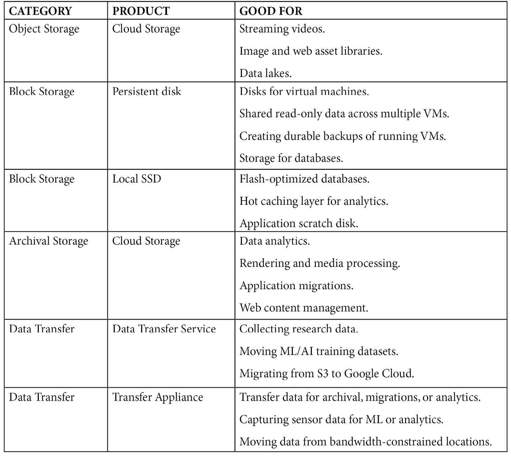
Additionally, Google offers the following information, which may help you understand the product you require:
Exam Tip
Understanding these options is critical. You may be presented with a scenario where relational databases are needed over non-relational databases, or where you need to select an option that is suitable for structured data. You also need to understand the limits of storage; as an example, let's say you are told that you need to assess a service that offers a NoSQL database and can scale to terabytes of data. After reading this article, you should be able to map this scenario to a service.
In the next section, we will discuss data consistency.
Data consistency
Data consistency refers to how the storage service handles transactions and how data is written to a database. As you go through this post, make sure that you review the consistency of each service, as this is one of the main design factors when choosing a product or service.
We will also take this chance to explain ACID. This is a key term in data consistency, and we will refer to this several times throughout this blog.
ACID is an acronym for the following attributes:
- Atomicity: This is where a transaction involves two or more pieces of information, and then all the pieces are committed or none at all are. For example, when performing a bank transfer, the debit and credit of the funds would be treated as a single transaction. If either the debit or credit fails, then both will fail.
- Consistency: If the aforementioned failure occurs, then all the data would be returned to the state before the transaction began.
- Isolation: The bank transfer would be isolated from any other transaction. In our example, this means that we would not debit from the bank until the transfer was complete.
- Durability: Even in the event of failure, the data would be available in its correct state.
Exam Tip
It's also important for you to be able to identify storage services that support structured data, low latency, or horizontal scaling. Likewise, you should be able to identify storage services that offer strong consistency or support ACID properties.
Now, let's look more closely at each of these services. We will begin with Cloud Storage.
Understanding Cloud Storage
Google Cloud Storage is a service for storing objects in Google Cloud. It is fully managed and can scale dynamically. Objects are referred to as immutable pieces of data consisting of a file of any format. Some use cases are video transcoding, video streaming, static web pages, and backups. It is designed to provide secure and durable storage while also offering optimal pricing and performance for your requirements through different storage classes.
Cloud Storage uses the concept of buckets; you may be familiar with this term if you have used AWS S3 storage. A bucket is a basic container where your data will reside and is attached to a GCP project, such as other GCP services. Each bucket name is globally unique and once created, you cannot change it. There is no minimum or maximum storage size, and we only pay for what we use. Access to our buckets can be controlled in several ways. We will learn more about security in This Post, Security and Compliance, but as an overview, we have the following main methods:
- Cloud Identity and Access Management (IAM): We will speak about IAM in more detail in This Article, Security and Compliance. IAM will grant access to buckets and the objects inside them. This gives us a centralized way to manage permissions rather than providing fine-grained control over individual objects. IAM policies are used throughout GCP, and permissions are applied to all the objects in a bucket.
- Access Control Lists (ACLs): ACLs are only used by Cloud Storage. This allows us to grant read or write access for individual objects. It is not recommended that you use this method, but there may be occasions when it is required. For example, you may wish to customize access to individual objects inside a bucket.
- Signed URLs: This gives time-limited read or write access to an object inside your bucket through a dedicated URL. Anyone who receives this URL can access the object for the time that was specified when the URL was generated.
We will also mention encryption in This Post, Security and Compliance. By default, Cloud Storage will always encrypt your data on the server side before it is written to disk. There are three options available for server-side encryption:
- Google-Managed Encryption Keys: This is where Cloud Storage will manage encryption keys on behalf of the customer, with no need for further setup.
- Customer-Supplied Encryption Keys (CSEKs): This is where the customer creates and manages their encryption keys.
- Customer-Managed Encryption Keys (CMEKs): This is where the customer generates and manages their encryption keys using GCP's Key Management Service (KMS).
There is also the client-side encryption option, where encryption occurs before data is sent to Cloud Storage and additional encryption takes place at the server side.
Bucket locations
Bucket locations allow us to specificity a location for storing our data. There are the following different location types:
- Region: This is a specific location, such as London.
- Dual-region: Dual-region is a pair of regions such as Iowa and South Carolina. Dual regions are geo-redundant, meaning that data is stored in at least two separate geographic places and will be separated by 100 miles, ensuring maximum availability for our data. Geo-redundancy occurs asynchronously.
- Multi-regions: A multi-region is a large area such as the EU and will contain two or more geographic places. Multi-regions are also geo-redundant. Of course, storing data in multiple locations will come at an increased cost.
Bucket locations are permanent, so some consideration should be taken before you select your preferred option. Data should be stored in a location that is convenient for your business users. For example, if you wish to optimize latency and network bandwidth for users in the same region, then region-based locations are ideal. However, if you also have additional requirements for higher availability, then consider dual-region to take advantage of this geo-redundancy.
Storage classes
We previously mentioned storage classes, and we should make it clear that it's vital to understand the different offerings to be successful in this exam. Let's take a look at these in more detail:
- Standard: This is the default setting for a new storage bucket. There is no minimum storage, and this is the best option for frequently accessed data and/or data that's only stored for small periods. When used alongside a multi- or dual region, the availability SLA for standard storage is 99.95%. When used in a single region, the availability SLA is 99.9%. Google also publishes what is known as typical monthly availability and for multi-region and dual-region this is > 99.99% while for regional, it is 99.99%.
- Nearline: Use the Nearline storage class for data that will be read or modified no more than once per month – for example, backup data. Nearline offers a slightly lower SLA than standard but this is a trade-off for lower at rest storage costs. When used alongside a multi- or dual region, the availability SLA for Nearline storage is 99.9% (the typical monthly availability is 99.95%). When used in a single region, then the availability SLA is 99.0% (the typical monthly availability is 99.9%). Nearline has very low cost-per-GB storage, but it does come with a retrieval cost. There is a 30-day minimum storage duration.
- Coldline: Use the Coldline storage class for data that is accessed no more than once per quarter; for example, for disaster recovery. It is a very low cost and highly durable service. When used alongside a multi- or dual region, the availability SLA for Coldline storage is 99.9% (the typical monthly availability is 99.95%). When used in a single region, then the availability SLA is 99.0% (the typical monthly availability is 99.9%). This class offers lower cost-per-GB storage than Nearline but comes with a higher retrieval cost. There is a 90-day minimum storage duration.
- Archive: Use Archive storage for long-term preservation of data that won't be accessed more than once a year. This is the lowest cost storage available and unlike many other cloud storage vendors, the data will be available in milliseconds rather than hours or days. There is a 365-day minimum storage duration. When used alongside a multi- or dual region, the typical monthly availability for archive storage is 99.95% with an SLA of 99.9%. When used in a single region, then the typical monthly availability is 99.9% with an SLA of 99.0%.
These different classes are summarized in the following diagram. Please note that the SLA and typical monthly availability may show different percentage values:
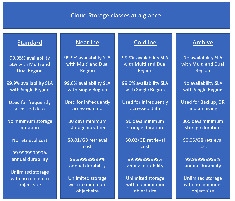
Figure 11.2 – Cloud Storage classes
You can edit Cloud Storage buckets to move between these storage classes. Note that there are additional storage classes that cannot be set using Cloud Console:
- Multi-region storage: This is equivalent to standard storage but can only be used for objects stored in multi-regions or dual regions.
- Regional storage: This is equivalent to standard storage but can only be used for objects stored in regions.
- Durable Reduced Availability (DRA) storage: This can be compared to standard storage but the DRA storage has a higher pricing for operations and a lower performance, especially in terms of availability, where it has an SLA of 99%.
Buckets get a default storage class upon their creation, and any objects inside it will inherit this class unless otherwise specified. We can change the default storage class of our bucket, but it will only apply to new objects after the change; the existing objects will remain in the original class. We can also effectively move data between buckets by using the Cloud Storage Transfer Service. However, note that moving data between locations incurs network usage costs. Additionally, we should be aware of extra costs that may be applicable. As Nearline, Coldline, and Archive storage are used to store infrequently accessed data, Google may apply retrieval or early deletion fees. A retrieval cost will be applied when we copy, read, or rewrite data or metadata that is stored in one of these storage classes.
Data consistency
Cloud Storage will provide both strong consistency and eventual consistency in certain circumstances.
Strong consistency can be expected in the following circumstances:
- When uploading data to Cloud Storage, meaning the data will always be available to read after a write or update operation.
- Once we delete the data successfully, the files will be instantly unavailable.
Eventual consistency can be expected in the following circumstance:
- When access to resources is revoked. It will typically take around 1 minute for access to be revoked, though in some cases, this may take even longer.
Cloud Storage FUSE
Cloud Storage cannot be mounted to a Google Compute Engine instance. However, if this is something that you would like to explore, GCP currently offers third-party integration using an open source FUSE adapter that will allow you to mount a storage bucket as a filesystem on Linux. This is available free of charge and is not officially supported; however, normal Cloud Storage charges are applicable.
Creating and using a bucket
Now that we have a good understanding of storage classes, let's take a look at how to create a bucket. We will also learn how to copy files into our bucket and change the storage policy of an object.
We have two options to create a bucket – either through a console or using gsutil. We will learn more about gsutil in This Post, Google Cloud Management Options, but for the context of this post, it's enough for you to know that it is a dedicated command-line tool that will make RESTful API calls to your Cloud Storage service. Let's look at how to create a bucket from the console by going through the following steps:
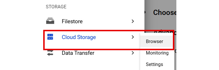
- Browse to STORAGE from the navigation menu. Then, select Cloud Storage | Browser:

Figure 11.3 – Navigating to Cloud Storage
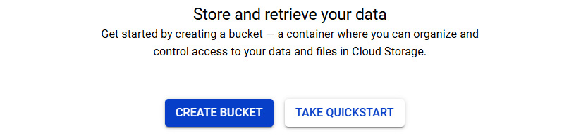
- Click on CREATE BUCKET, as shown in the following screenshot:

Figure 11.4 – CREATE BUCKET
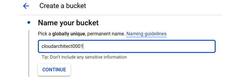
- Give the bucket a name. Remember that this must be globally unique:

Figure 11.5 – Name your bucket
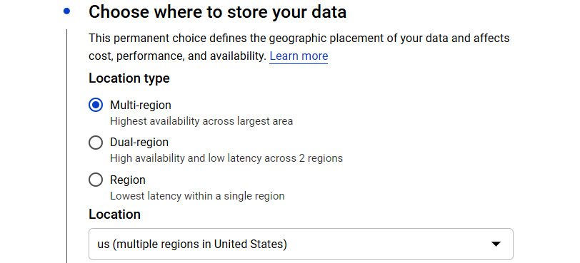
- Select the location for your bucket:

Figure 11.6 – Location type
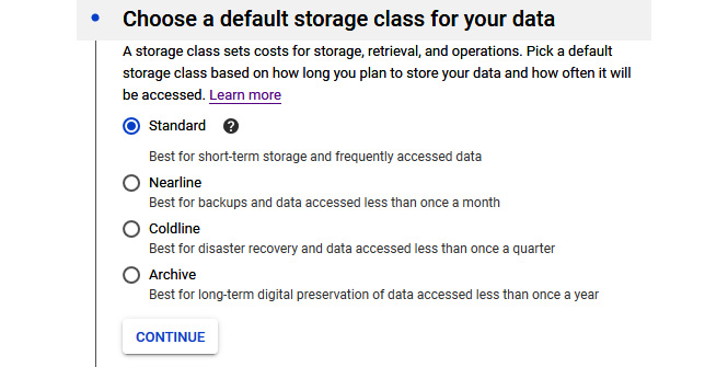
- Select a storage class that fits your needs. Select a location. You will notice that the location will either be a zone or a region, depending on whether your selection is Multi-region or Region. Bear in mind that your selection will have an impact on the cost:

Figure 11.7 – Storage class options
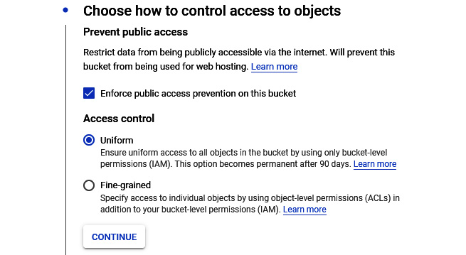
- Select either an ACL or IAM access control model:

Figure 11.8 – Access control options
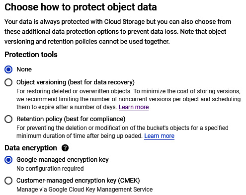
- We can also set more advanced settings that will show the encryption and retention policies. By default, Google will manage our keys. A retention policy can also be set. This will offer a minimum duration in which objects in the bucket will be protected from deletion:

Figure 11.9 – Optional advanced settings
- Click Create and we are done.
As you can see, this is a pretty simple process. Let's make it even simpler by creating it from our dedicated command-line tool, gsutil, which we can access from Cloud Shell:
- In Cloud Shell, we can run the following command:
gsutil mb -c <storage class> -l <location> gs://<bucket name>
Let's look at the code in a little more detail:
- <storage class> is the class we would like to apply to our bucket.
- <location> is the region we want to create our bucket in.
- <bucket name> is the unique name we want to assign to our bucket.
- Let's create a new bucket called cloudarchitect001 in the us-east1 region and apply the regional storage class:
gsutil mb -c regional -l us-east1 gs://cloudarchitect001
- Now, we have a bucket with no data inside. Let's use gsutil and move some objects into our bucket with the following syntax:
gsutil cp <filename> gs://<bucketname>
Here, <filename> is the name of the file you wish to copy, while <bucketname> is the destination bucket.
- In this example, let's copy over a file called conf.yaml to our new bucket, called cloudarchitect001:
gsutil cp conf.yaml gs://cloudarchitect001
- Let's look at how to change the storage class of a file. The storage class of an individual object can only be put inside a bucket using gsutil. We should use the following syntax:
gsutil rewrite -s <storage class> gs://<bucket name>/<file name>
- Let's change our file, conf.yaml, so that it uses Coldline storage:
gsutil rewrite -s coldline gs://cloudarchitect001/conf.yaml
Great! So, we now know how to manage our buckets. In the next section, we will take a look at some key features of Cloud Storage.
Versioning and life cycle management
Now, let's take a look at versioning and life cycle management. These are important features offered by Cloud Storage and are of particular significance for the exam.
Exam Tip
Cloud Storage offers an array of features. To succeed in the exam, you must understand the versioning and life cycle management features of Cloud Storage. Like the storage classes, you should review these and make sure you are comfortable before moving on to future sections of this article.
Versioning
Versioning can be enabled to retrieve objects that we have deleted or overwritten. Note that, at this point, this will increase storage costs, but this may be worth it for you to be able to roll back to previous versions of important files. The additional costs come from the archived versions of each object that is created each time we overwrite or delete the live version of an object. The archived version of the file will retain the original name but will also be appended by a generation number to identify it. Let's go through the process of versioning:
- To enable versioning, we should use the gsutil command:
gsutil versioning set on gs://<bucket name>
Here, <bucket name> is the bucket that we want to enable versioning on.
Let's look at the following screenshot, which shows how this looks. In this example, we are enabling versioning on our cloudarchitect bucket and then confirming that versioning is indeed enabled:

Figure 11.10 – Set versioning
- Now, let's copy a file called vm.yaml to our bucket. We can use the -v switch to version it:

Figure 11.11 – Copying the file
- If we modify this file, we can list the available versions by running a command with the following syntax:
gsutil ls -a gs://<bucket name>/<filename>
Let's run this command on our file, named vm.yaml, which resides in our cloudarchitect bucket. We can see that we have several archived versions available:


Figure 11.12 – Viewing the different versions
We can turn versioning on and off whenever we want. Any available archived versions will remain when we turn it off, but we should remember that we will not have any archived versions until we enable this option.
Life cycle management
Archived files could quickly get out of hand and impact our billing unnecessarily. To avoid this, we can utilize life cycle management policies. Life cycle management configurations can be assigned to a bucket. These files are a set of rules that can be applied to current or future objects in the bucket. When any of the objects meet the guidelines of the configuration, Cloud Storage can perform actions automatically.
One of the most common use cases for using life cycle management policies is when we want to downgrade the storage class of objects after a set period. For example, there may be a scenario where data needs to be accessed frequently up to 30 days after it is moved to Cloud Storage, and after that, it will only be accessed once a year. It makes no sense to keep this data in regional or multi-regional storage, so we can use life cycle management to move this to Coldline storage after 30 days. Perhaps objects are not needed at all after 1 year, in which case we can use a policy to delete these objects. This helps keep costs down. Let's learn how we can apply a policy to a bucket.
The first thing we need to do is create a life cycle configuration file. As we mentioned previously, these files contain a set of rules that we want to apply to our bucket. If the policy contains more than one rule, then an object has to match all of the conditions before the action will be taken. It might be possible that a single object could be subject to multiple actions; in this case, Cloud Storage will perform only one of the actions before re-evaluating any additional actions.
We should also note that a Delete action will take precedence over a SetStorageClass action. Additionally, if an object has two rules applied to it to move the object to Nearline or Coldline, then the object will always move to the Coldline storage class if both rules use the same condition. A configuration file can be created in JSON or XML.
In the following example, we will create a simple configuration file in JSON format that will delete files after 60 days. We will also delete archived files after 30 days. Let's save this as lifecycle.json:
{
"lifecycle": {
"rule": [{
"action": {
"type": "Delete"
},
"condition": {
"age": 60,
"isLive": true
}
}, {
"action": {
"type": "Delete"
},
"condition": {
"age": 30,
"isLive": false
}
}]
}
}
Exam Tip
If the value of isLive is true, then this lifecycle condition will only match objects in a live state; however, if the value is set to false, the lifecycle condition will only match archived objects. We should also note that objects in non-versioned buckets are considered live.
We can also use gsutil to enable this policy on our buckets using the following syntax:
gsutil lifecycle set <lifecycle policy name> gs://<bucket name>
Here, <lifecycle policy name> is the file we have created with our policy, while <bucket name> is the unique bucket name we want to apply the policy to. The following code shows how to apply our lifecycle.json file to our cloudarchitect bucket:
gsutil lifecycle set lifecycle.json gs://cloudarchitect
We mentioned earlier that a common use case for lifecycle would be to move objects to a cheaper storage class after a set period. Let's look at an example that would map to a common scenario. Suppose we have objects in our cloudarchitect bucket that we want to access frequently for 90 days. After this time, we only need to access the data monthly. Finally, after 180 days, we will only access the data yearly. We can translate these requirements into storage classes and create the following policy, which will help keep our costs to a minimum.
Let's break this down a little since we now have a policy with two rules that each have two conditions. Any storage object with an age greater than 90 days and that has the REGIONAL storage class applied to it will be moved to NEARLINE storage. Any object with an age greater than 180 days and that has the NEARLINE storage class applied to it will be moved to ARCHIVE storage:
{
"lifecycle": {
"rule": [{
"action": {
"type": "SetStorageClass",
"storageClass": "NEARLINE"
},
"condition": {
"age": 90,
"matchesStorageClass": ["REGIONAL"]
}
},
{
"action": {
"type": "SetStorageClass",
"storageClass": "ARCHIVE"
},
"condition": {
"age": 180,
"matchesStorageClass": ["NEARLINE"]
{
Exam Tip
At least one condition is required. If you enter an incorrect action or condition, then you will receive a 400 bad request error response.
Next, let's check out retention policies and locks.
Retention policies and locks
Bucket locks allow us to configure data retention policies for a Cloud Storage bucket. This means we can govern how long objects in the bucket must be retained and prevent the policy from being reduced or removed.
We can create a retention policy by running the following command:
gsutil retention set 60s "gs://<bucketname>"
This sets the policy for 60 seconds. We can also set it to 60d for 60 days, 1m for 1 month, or 10y for 10 years. The output of setting this policy will be similar to the following:
Retention Policy (UNLOCKED):
Duration: 60 Second(s)
Effective Time: Thu, 01 Jul 2021 05:49:05 GMT
Note that if a bucket does not have a retention policy, then we can delete or replace objects at any time. However, if a policy is applied, then the objects in the bucket can only be replaced or deleted once their age is older than the retention policy period.
Exam Tip
Retention policies and object versioning are exclusive features, which means that for a given bucket, only one of these can be enabled at a time.
Object holds
Object holds are metadata flags that can be placed on individual objects, which means they cannot be replaced or deleted. We can, however, still edit the metadata of an object that has been placed on hold.
There are two types of holds and an object can have one, both, or neither hold applied. When an object is stored in a bucket without a retention policy, both hold types behave in the same way. However, if a retention policy has been applied to the bucket, the holds have different effects on an object when the hold is released:
- Event-based hold: This resets the object's time in the bucket for the retention period.
- Temporary hold: This does not affect the object's time in the bucket for the retention period.
Let's look at an example to make things a little clearer. Let's say we have two objects – Object A and Object B – that we add to a storage bucket that has a 1-month retention period. We apply an event-based hold on Object A and a temporary hold on Object B. Due to the retention period alone, we would usually be able to delete both objects after 1 month. However, because we applied an object hold to each object, we are unable to do so. If we release the hold on Object A, then due to the event-based hold, the object must remain in the bucket for another 1 month before we can delete it. If we release the hold on Object B, we can immediately delete this due to the temporary hold not affecting the object's time in the bucket.
Transferring data
There will be cases where we want to transfer files to a bucket from on-premises or another cloud-based storage, and Google offers many ways to do so. There are some considerations that we should bear in mind to make sure that we select the right option. The size of the data and the available bandwidth will be the deciding factors. Let's take a quick look at a chart to show how long it would take to transfer some set data sizes over a specific bandwidth:
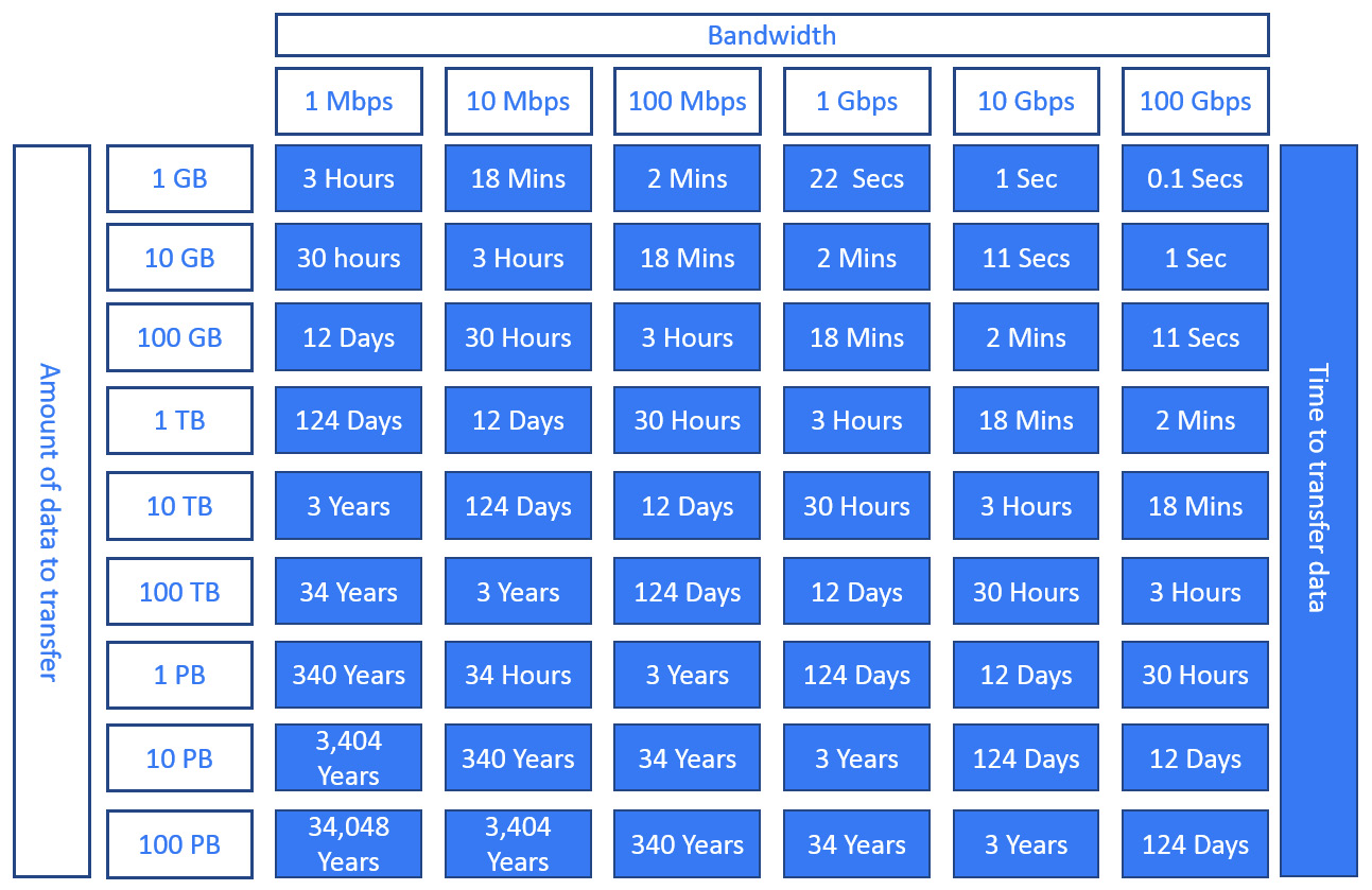
Figure 11.13 – Data transfer guidance
Next, Let's look at some methods of transferring data.
Cloud Storage Transfer Service
Cloud Storage Transfer Service provides us with the option to transfer or back up our data from online sources to a data sink. Let's say, for example, that we want to move data from our AWS S3 bucket into our Cloud Storage bucket. S3 would be our source and the destination Cloud Storage bucket would be our data sink. We can also use Cloud Storage Transfer Service to move data from an HTTP/HTTP(s) source or even another Cloud Storage bucket. To make these data migrations or synchronizations easier, Cloud Storage Transfer Service offers several options:
- We can schedule a one-time transfer operation or a recurring operation.
- We can delete existing objects in the destination data sink if they don't have any corresponding objects in the source.
- We can delete source objects once we have transferred them.
- We can schedule periodic synchronizations between the source and destination using folders based on file creation dates, filenames, or even the time of day you wish to import data.
Exam Tip
You can also use gsutil to transfer data between Cloud Storage and other locations. You can speed up the process of transferring files on-premises by using the -m option to enable a multi-threaded copy. If you plan to upload larger files, gsutil will split these files into several smaller chunks and upload these in parallel.
It is recommended that you use Cloud Storage Transfer Service when transferring data from Amazon S3 to Cloud Storage.
Google Transfer Appliance
If we look at Figure 9.13, we can see that there are some pretty large transfer times. If we have petabytes of storage to transfer, then we should use Transfer Appliance. This is a hardware storage device that allows secure offline data migration. It can be set up in our data center and is rack-mountable. We simply fill it with data and then ship it to an ingest location where Google will upload it to Cloud Storage.
Google offers the option of a 40 TB or 300 TB transfer appliance. The following is a quote from https://cloud.google.com/transfer-appliance/docs/4.0/security-and-encryption:
A common use case for Transfer Appliance is to move large amounts of existing backups from on-premises to cheaper Cloud Storage using the Coldline storage class. It would take more than 1 week to perform this upload over the network.
Now, we will have a look at IAM.
Understanding IAM
Access to Google Cloud Storage is secured with IAM. Let's have a look at the following list of predefined roles and their details:
- Storage Object Creator: Has rights to create objects but does not give permissions to view, delete, or overwrite objects
- Storage Object Viewer: Has rights to view objects and their metadata, but not the ACL, and has rights to list the objects in a bucket
- Storage Object Admin: Has full control over objects and can create, view, and delete objects
- Storage Admin: Has full control over buckets and objects
- Storage HMAC Key Admin: Has full control over HMAC keys in a project and can only be applied to a project
Quotas and limits
Google Cloud Storage comes with predefined quotas. These default quotas can be changed via the Navigation menu, under the IAM & Admin | Quotas section. From this menu, we can review the current quotas and request an increase to these limits. We recommend that you familiarize yourself with the limits of each service as this can have an impact on your scalability. For Cloud Storage, we should be aware of the following limits:
- Individual objects are limited to a maximum size of 5 TiB.
- Updates to an individual object are limited to one per second.
- There is an initial limit of 1,000 writes per second per bucket.
- There is an initial limit of 5,000 reads per second per bucket.
- There is a limit of 100 ACL entries per object.
- There is a limit of one bucket creation operation every 2 seconds.
- There is a limit of one bucket deletion operation every 2 seconds.
Pricing
Pricing for Google Cloud Storage is based on four components:
- Data storage: This applies to at-rest data that is stored in Cloud Storage, is charged per GB per month, and the cost depends on the location and class of the storage.
- Network usage: This applies when object data or metadata is read from or moved between our buckets.
- Operations usage: This applies when you perform actions within Cloud Storage that make changes or retrieve information about buckets and their objects. The cost depends on the class of the storage.
- Retrieval and early deletion fees: This applies when accessing data from the Nearline, Coldline, and Archive storage classes. Retrieval costs will apply when we read, copy, or rewrite data or metadata. The minimum storage duration applies to data stored in Nearline, Coldline, and Archive storage. You will still be charged for the duration of an object, even if the file is deleted before the minimal period.
Understanding Cloud Firestore
It's wise to note early on in this section that Google rebranded their previous Cloud Datastore product with a newer major version called Cloud Firestore. However, it is also important to understand the relationship between both as Firestore gives the option of Native mode and Datastore mode, with the latter using the traditional Datastore system's behaviors with the Firestore storage layer, which eliminates some of Datastore's limitations.
Cloud Datastore is a NoSQL database that is built to ease application development. It uses a distributed architecture that is highly scalable, and because it is serverless, we do not have to worry about the underlying infrastructure. Cloud Datastore distributes our data over several machines and uses masterless, synchronous replication over a wide geographical area.
Firestore builds on this but also accelerates the development of mobile, IoT, and web applications. It offers built-in live synchronization, as well as an offline mode that increases the efficiency of developing real-time applications. This includes workloads consisting of live asset tracking, real-time analytics, social media profiles, and gaming leaderboards.
Firestore also offers very high availability (HA) on our data. With automatic multi-region replication and strong consistency, it offers a 99.999% guarantee.
Before we go any further into the details, we don't want to make any assumptions that you know what a NoSQL database is. SQL databases are far more well-known by non-database administrators in the industry. A SQL database is primarily a relational database that is based on tables consisting of several rows of data that have predefined schemas.
Compare that to the concept of a NoSQL database, which is a non-relational database based around key-value pairs that do not have to adhere to any schema definitions. Ultimately, this allows us to scale efficiently; therefore, we can see how it becomes a lot easier to add or remove resources as we need to. This elasticity makes Cloud Datastore perfect for transactional information, such as real-time inventories, ACID transactions that will always provide data that is valid, or for providing user profiles to keep a record of user experience based on past activities or preferences. However, it is also important to note that NoSQL databases may not be the perfect fit for every scenario and consideration should be taken when deciding on what database to select, particularly regarding the efficiency of querying your data. OK; so, now that we know what a NoSQL database is, let's look at what makes up a Datastore database, as relationships between data objects are addressed differently than other databases that you may be familiar with. A traditional SQL database would be made up of tables, rows, and columns. In Cloud Datastore, an entity is the equivalent of a row, and a kind is the equivalent of a table. Entities are data objects that can have one or more named properties.
Each entity has a key that identifies it. Let's look at the following table to compare the terminology that is used with SQL databases and Cloud Datastore:
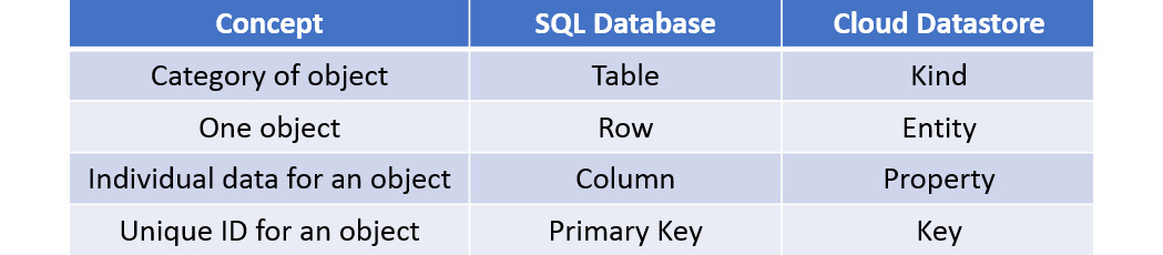
Figure 11.14 – Terminology comparison
Now, let's look at the different types of modes that are offered in more detail.
Cloud Firestore in Datastore mode or Native mode
When we create a new database, we must select one of the modes. However, we cannot use a mixture of modes within the same project. So, it is recommended to think about your design and what your application is built for.
Native mode offers all the new features of the revamped product. It takes the best of Cloud Datastore and the Firebase real-time database. Firebase was originally designed for mobile applications that required synced states across clients in real time. As such, Firestore takes advantage of this and offers a new, strongly consistent storage layer, as well as real-time updates. Additionally, it offers a collection and document data model and mobile and web client libraries. Native mode can scale automatically to millions of concurrent clients.
Exam Tip
While Firestore is backward compatible with Datastore, the new data model, real-time updates, and mobile and web client libraries are not. You must use Native mode to gain access to these features.
Datastore mode supports the Datastore API, so there is no requirement to change any existing Datastore applications. If your architecture requires the use of an established Datastore server architecture, then Datastore mode allows for this and removes some of the limitations from Datastore, mainly that Datastore mode offers strong consistency unless eventual consistency is specified. Datastore mode can scale automatically to millions of writes per second.
Exam Tip
Data objects in Firestore in Datastore mode are known as entities.
Upgrading to Firestore
New projects that require a Datastore database should use Firestore in Datastore mode. However, starting in 2021, existing Datastore databases will be automatically upgraded without the need to update your application code. Google will notify users of the schedule for the upgrade, which does not require downtime.
Creating and using Cloud Datastore
The first thing we need to do is select a mode before we can utilize Cloud Firestore. Let's look at creating a database in Datastore mode and run some queries on the entities that we create. Before we do so, let's remind ourselves that Datastore is a managed service. As we go through this process, you will note that we are directly creating our entities without provisioning any underlying infrastructure first. You should also note that, like all storage services from GCP, Cloud Datastore automatically encrypts all data before it's written to disk. Follow these steps to create a Firestore in Datastore mode:
- From our GCP Console, browse to DATABASES Firestore:

Figure 11.15 – Selecting Firestore
- We are now required to choose an operational mode. Native mode is the official Firestore mode, which is the next major version of Cloud Datastore and offers new features, such as real-time updates and mobile and web client libraries. Datastore mode uses traditional Cloud Datastore system behavior. In our example, we will use Datastore mode:

Figure 11.16 – Choosing Datastore mode
- Select a location for your Datastore database and click CREATE DATABASE:

Figure 11.17 – Selecting a location
- Once the database is ready, we will be directed to the Entities menu. Click CREATE ENTITY to create our first Datastore entity:

Figure 11.18 – Creating an entity
We can now give our entity a namespace, a Kind (a table, in SQL terminology), and a key identifier, which will be auto-generated. Let's leave our namespace as the default and create a new kind called exam:

Figure 11.19 – Create an entity
- Click ADD PROPERTY to specify a name – in this case, title. We can also select from several types, but in this example, we want to use String. Finally, we will give it the value of Professional Cloud Architect. Click DONE to add the property:

Figure 11.20 – Adding entity properties
- We can repeat Step 5 to add another property. This time, we will use cost as the name, Integer as the type, and 200 as the value. When we have added all of the properties we want in our entity, click CREATE. Let's also create two new entities with the exam kinds for the Associate Cloud Engineer exam and the Professional Cloud Developer exam:

Figure 11.21 – Creating an entity
- Now, we can filter our entities to a query based on cost or title. Let's look for information on the Professional Cloud Developer exam:

Figure 11.22 – Filter entities
- We can also use QUERY BY GQL and enter a SQL-like query to get the same results:

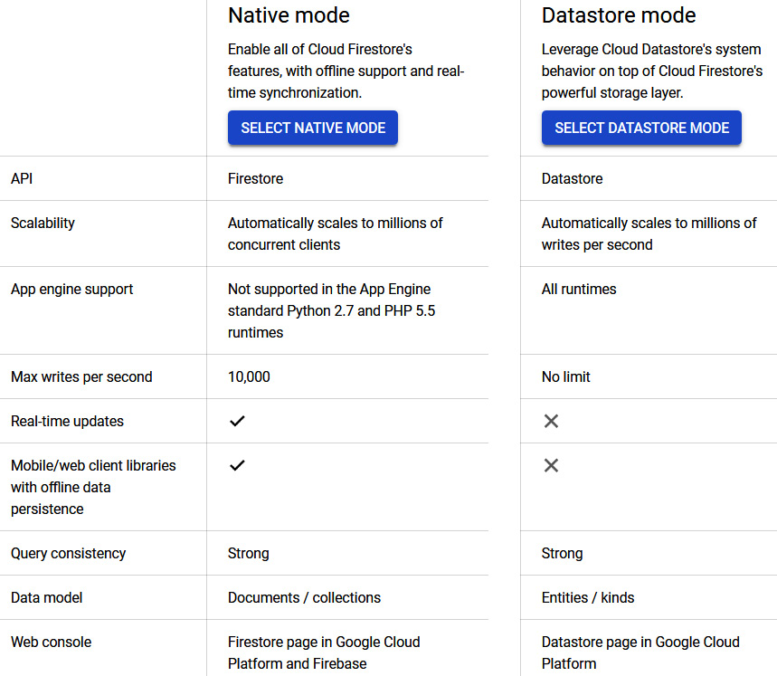
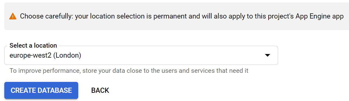

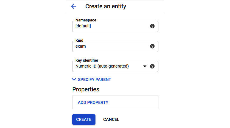
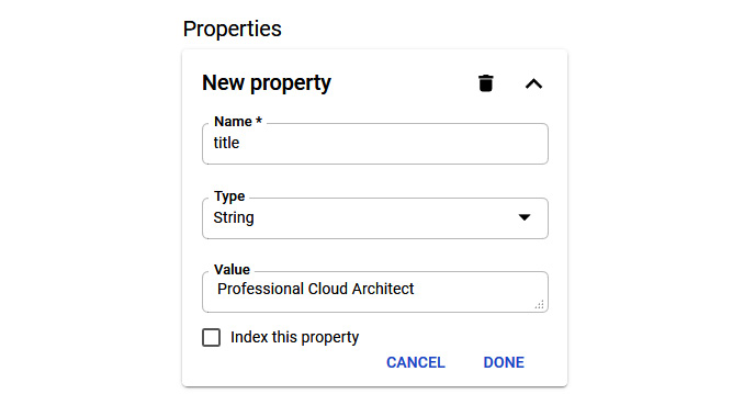
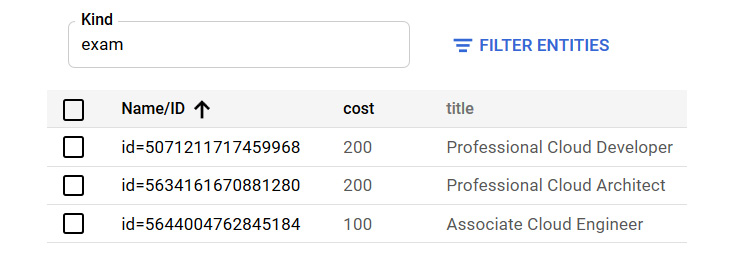
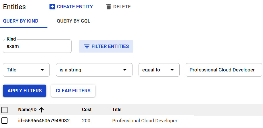
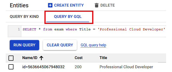
Figure 11.23 – Executing the query
With that, we have seen how easy it is to create a Datastore database and query the entities we create. Now, let's move on and look at some of the differences between Datastore and Firestore.
Summary of Datastore mode versus Native mode
Cloud Firestore in Native mode is the complete re-branded product. It takes the best of Cloud Datastore and the Firebase real-time database to offer the same conceptual NoSQL database as Datastore, but as Firebase is built for low-latency mobile applications, it also includes the following new features:
- A new strongly consistent storage layer
- A collect and document data model
- Real-time updates
- Mobile and web client libraries
Cloud Firestore in Datastore mode uses the same Datastore system behavior but will access the Firestore storage layer, which will remove some limitations, such as the following:
- No longer limited to eventual consistency, as all queries become strongly consistent
- No longer limited to a 25 entity group limit
- No longer limited to 1 write per second to an entity group
IAM
Access to Google Cloud Datastore is secured with IAM. Let's have a look at the list of predefined roles and their details:
- Datastore owner with an AppEngine app admin: Has full access to Datastore mode
- Datastore owner without an AppEngine app admin: Has access to Datastore mode but cannot enable admin access, check whether Datastore mode admin is enabled, disable Datastore mode writes, or check whether Datastore mode writes are disabled
- Datastore user: Has read/write access to data in a Datastore mode database. Mainly used by developers or service accounts
- Datastore viewer: Has rights to read all Datastore mode resources
- Datastore import-export admin: Has full access to manage imports and exports
- Datastore index admin: Has full access to manage index definitions
Quotas and limits
Google Cloud Datastore comes with predefined quotas. These default quotas can be changed by going to the Navigation menu, under the IAM & Admin | Quotas section. From this menu, we can review the current quotas and request an increase to these limits. We recommend that you familiarize yourself with the limits for each service as this can have an impact on your scalability. Cloud Firestore offers a free quota that allows us to get started at no cost:
- There is a 1 GiB limit on stored data.
- There is a limit of 50,000 reads per day.
- There is a limit of 20,000 writes per day.
- There is a limit of 20,000 deletes per day.
- There is a network egress limit of 10 GiB per month.
With the free tier, there are the following standard limits:
- There is a maximum depth of subcollections of 100.
- There is a maximum document size of 6 KiB.
- There is a maximum document size of 1 MiB.
- There is a maximum writes per second per database of 10,000.
- There is a maximum API request size of 10 MiB.
- There is a maximum of 500 writes that can be passed to a commit operation or performed in a transaction.
- There is a maximum of 500 field transformations that can be performed on a single-document Commit operation or in a transaction.
Pricing
Pricing for Google Cloud Firestore offers a free quota to get us started, as mentioned previously.
If these limits are exceeded, there will be a charge that will fluctuate, depending on the location of your data. General pricing is per 100,00 documents for reads, writes, and deletes. Stored data is charged per GB per month.
Understanding Cloud SQL
Given the name, it won't be a major surprise to hear that Cloud SQL is a database service that makes it easy to set up, maintain, and manage your relational PostgreSQL, MySQL, or SQL Server database on Google Cloud.
Although we are provisioning the underlying instances, it is a fully managed service that is capable of handling up to 64 TB of storage. Cloud SQL databases are relational, which means that they are organized into tables, rows, and columns. As an alternative, we can install the SQL Server application image onto a Compute Engine instance, but Cloud SQL offers many benefits that come from being fully managed by Google – for example, scalability, patching, and updates are applied automatically, automated backups are provided, and it offers HA out-of-the-box. Again, it is important to highlight that although these benefits may look great, we should also be mindful that there are some unsupported functions and that consideration should be taken before committing to Cloud SQL.
Exam Tip
Cloud SQL can accommodate up to 64 TB of storage. If you need to handle larger amounts of data, then you should look at alternative services, such as Cloud Spanner.
Now, let's look at some of the features offered by Cloud SQL.
Cloud SQL for MySQL offers us the following:
- MySQL currently offers support for MySQL 5.6, 5.7, and 8.0 and can provide up to a maximum of 624 GB of RAM and 64 TB of storage when selecting a high memory instance type.
- There's data replication between multiple zones with automatic failover.
- Fully managed MySQL Community Edition databases are available in the cloud.
- There's point-in-time recovery and on-demand backups.
- There's instance cloning.
- It offers integration with GCPs monitoring and logging solutions – Cloud Operations.
Cloud SQL for PostgreSQL offers us the following:
- A fully managed PostgreSQL database in the cloud with up to 64 TB of storage, depending on whether the instance has dedicated or shared vCPUs
- Custom machine types with up to 624 GB RAM and 96 CPUs
- Data replication between multiple zones with automatic failover
- Instance cloning
- On-demand backups
- Integration with GCPs monitoring and logging solutions – Cloud Operations logging and monitoring
Cloud SQL for SQL Server offers us the following:
- A fully-managed SQL Server database in the cloud.
- Custom machine types with up to 624 GB RAM and 96 CPUs.
- Up to 64 TB of storage.
- Custom data encrypted in Google's internal networks and database tables, temporary files, and backups.
- Databases can be imported using BAK and SQL files.
- Instance cloning.
- Integration with Cloud Operations logging and monitoring.
- Data replication between multiple regions.
- HA through regional persistent disks.
Now that we know the main features, let's look at some of the things to bear in mind when we create a new instance:
- Selecting an instance: Similar to other GCP services, we have the option to select a location for our instances. It makes sense to place our database instance close to the services that depend on it. We should understand our database requirements and have a baseline of active connections, memory, and CPU usage to allow us to select the correct machine type. If we over-spec, this will have an impact on our cost, and likewise, if we under-spec, we may impact our performance or availability if resources are exhausted.
- Selecting region: We have the option to select the region that our instance will be deployed to. Be mindful that the region cannot be changed after deployment, but the zone can be changed at any time. For HA, we can select multiple zones, which offers automatic failover to another zone in our selected region. From a performance standpoint, we should be looking to deploy our instances close to the services that are using them. We will look at HA in more detail later in this blog.
- Selecting storage: When creating an instance, we can select different storage tiers. Depending on our requirements, we may wish to select an SSD for lower latency and higher throughput; however, we can also select an HDD if we don't require such a high-performing disk.
- Selecting encryption: When creating an instance, we can choose to have Google manage our encryption keys, which is the default, or select a customer-managed key, which is managed via the Google KMS service.
Selecting the correct capacity to fit your database size is also extremely important because once you have created your instance, you cannot decrease the capacity. If we over-spec our storage, then we will be paying for unused space. If we under-spec our storage, then we can cause issues with availability. One method to avoid this is through the automatic storage increase setting. If this is enabled, your storage is checked every 30 seconds to ensure that the storage has not fallen below a set threshold size. If it has, then additional storage will be automatically added to your instance. The threshold's size depends on the amount of storage your instance currently has provisioned, and it cannot be larger than 25 GB. This sounds great, but we should also be mindful that if we have spikes in demand, then we will suffer a permanent increase in storage cost. We should also be mindful that creating or increasing storage capacity to 30 TB or greater could lead to increased latency for operations such as backups:
- Selecting an IP address: We can select from a public or a private IP address. The default is to use a public IP address, which will block all IP addresses. So, we must add specific IP addresses or ranges to open our instances up. To use a private IP address, we must enable Google's Service Networking API. This is required for each project. If we wish to use a private IP address, we need to ensure that we have VPC peering set up between the Google service VPC network where our instance resides and our VPC network. This is shown in the following diagram:
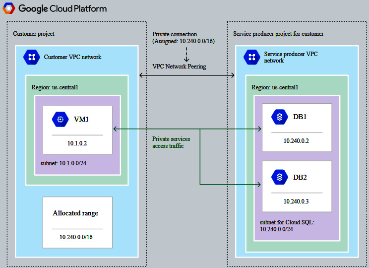
Figure 11.24 – VPC peering (Source: https://cloud.google.com/sql/docs/postgres/private-ip. License: https://creativecommons.org/licenses/by/4.0/legalcode)
We discussed VPC peering in more detail in This Post, Networking Options in GCP. Using a private IP will help lower network latency and improve security as traffic will never be exposed to the internet; however, we should also note that to access a Cloud SQL instance on its private IP address from other GCP resources, the resource must be in the same region.
Important Note
It is recommended that you use a private IP address if you wish to access a Cloud SQL instance from an application that is running in Google's container service; that is, Google Kubernetes Engine.
- Automatic backups: Enabling automatic backups will have a small impact on performance; however, we should be willing to accept this to take advantage of features such as read replicas, cloning, or point-in-time recovery. We can select where our backups are located. However, by default, backups are stored in the closest multi-region location, so they should only be customized based on unique design decisions. Additionally, we can select how many automatic backups are stored. This defaults to 7 and again, unless there is a specific reason to change this, then it is not recommended to modify it. Also, please note that if multiple zones are selected, then automatic backups are enabled by default and cannot be disabled.
- Maintenance windows: When working with this offering, we should also specify a maintenance window. We can choose a specific day and 1-hour time slot when updates can be applied. GCP will not initiate any update to that instance within this specified window. Please note that if no window is specified, then potentially disruptive updates can occur at any time.
Data consistency
Cloud SQL is a relational database that offers strong consistency and support for ACID transactions.
Creating and managing Cloud SQL
Now that we have an understanding of the concepts, let's look at how to create a new MySQL instance:
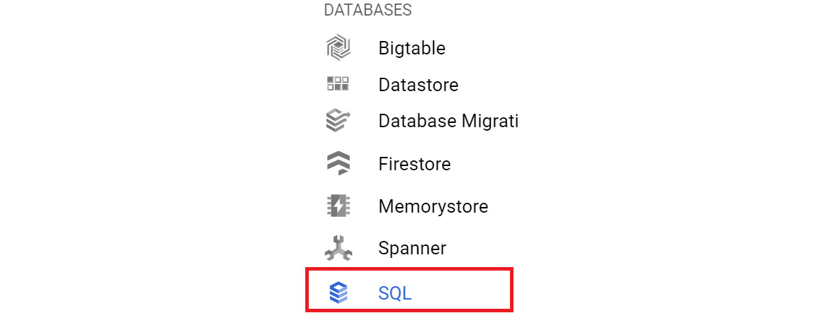
- Go to the navigation menu and go to DATABASES | SQL:

Figure 11.25 – Selecting SQL
- Click on Create an instance.
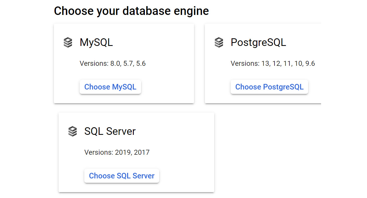
- Select the database engine you require. In our example, we will select MySQL:

Figure 11.26 – Choose your database engine
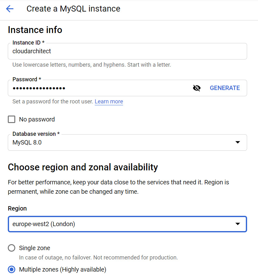
- Give the instance a name and a password. You can either enter your own password or click Generate to receive a random password. Additionally, you can select a location and database version. We will leave the defaults in this example as-is:

Figure 11.27 – Create a MySQL instance
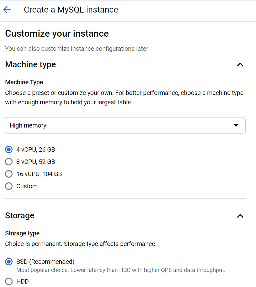
- Now, let's look at some of the custom configurations. First, we must select our machine type and storage options:

Figure 11.28 – Selecting the machine type and storage
We can also set the storage capacity and encryption options to enable the use of customer-managed encryption keys. In the preceding screenshot, we are using the default settings.
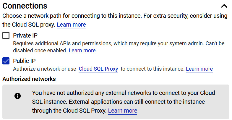
- Next, we can choose whether we want a private or public IP address for our instance:

Figure 11.29 – Selecting a connection type
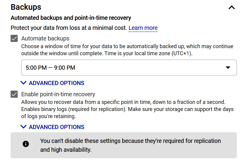
- Provide 4 hours for a backup. Also, ensure that you check the Create failover replica option if required:

Figure 11.30 – Creating a backup schedule
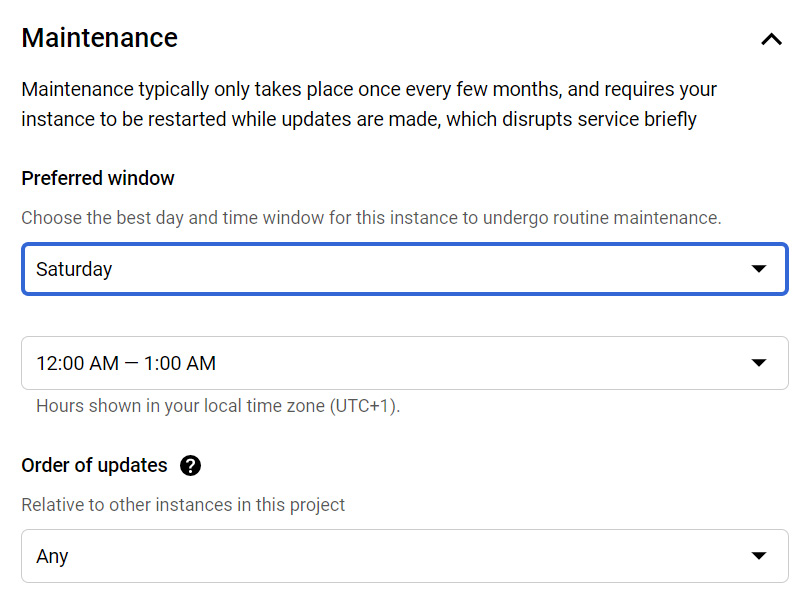
- Set a maintenance schedule by selecting a day and 1-hour time slot:

Figure 11.31 – Creating maintenance windows
- At this point, we can also add any labels we require. Finally, click CREATE.
Like other services, we can create an instance by using the command-line tools available to us. Earlier in this post, we touched on some command-line tools, and likewise, we can use gcloud to create a new instance. We can run the following syntax to create a new database:
gcloud sql instances create <instance name> --database-version=<DATABASE version> --cpu=<cpu size> --memory=<RAM size> --region=<region name>
Let's look at this code in a little more detail:
- <instance name> is the name of our database instance.
- <DATABASE version> is the name of the specific version of MySQL or PostgreSQL you wish to create.
- <cpu size> and <RAM size> are the sizes of the resources we wish to create.
- <region name> is the region we wish to deploy our instance to.
Let's create a new PostgreSQL DB with version 9.6 called cloudarchitect001 and allocate 4 CPUs and 3,840 MiB of RAM. We will deploy this instance in the us-central region. Please note that this command may ask you to enable the API. Click Yes:
gcloud sql instances create cloudarchitect001 --database-version=POSTGRES_9_6 --cpu=1 --memory=3840MiB --region=us-central
Exam Tip
You can directly map your on-premises MySQL, SQL, or PostgreSQL database to Cloud SQL without having to convert it into a different format. This makes it one of the common options for companies looking to experiment with public cloud services.
Now that we have created a new instance by console and command line, let's look at some important features in more detail – read replicas and failover replicas.
Read replicas
Cloud SQL offers the ability to replicate our master instance to one or more read replicas. This is essentially a copy of the master that will register changes that are made to the master in the replica in almost real time.
Tip
We should highlight here that read replicas do not provide HA, and we cannot failover to a read replica from a master. They also do not fall in line with any maintenance window that we may have specified when creating the master instance.
There are several scenarios that Cloud SQL offers for read replication:
- Read replica: This offers additional read capacity and an analytics target to optimize performance on the master.
- Cross-region read replica: This offers the same as a standard read replica but also offers disaster recovery capabilities, improved read performance, and the ability to migrate between regions.
- External read replica: This replicates to a MySQL instance that is external to Cloud SQL. It can help reduce latency if you are connecting from an on-premises network and also offers a migration path to other platforms.
- Replication from an external server: This is where an external MySQL instance is the master and is being replicated into Cloud SQL. This also offers data replication to GCP.
Enabling read replicas is a simple process. Let's learn how to do this from our GCP Console:
- Browse once more to Database | SQL. Let's add a replica to our existing cloudarchitect001 instance. We simply need to open our options menu and select Create read replica:

Figure 11.32 – Create read replica
Exam Tip
Before we can create a read replica, the following requirements must be met: binary logging must be enabled and at least one backup must have been created since binary logging was enabled.
Simply give the instance a name, select a region, and click Create. We will see configuration options similar to those we used when we created a master instance:

Figure 11.33 – Creating a replica
- Once the read replica has been created, we will see the following in our normal instance view:
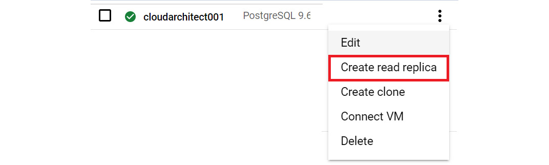
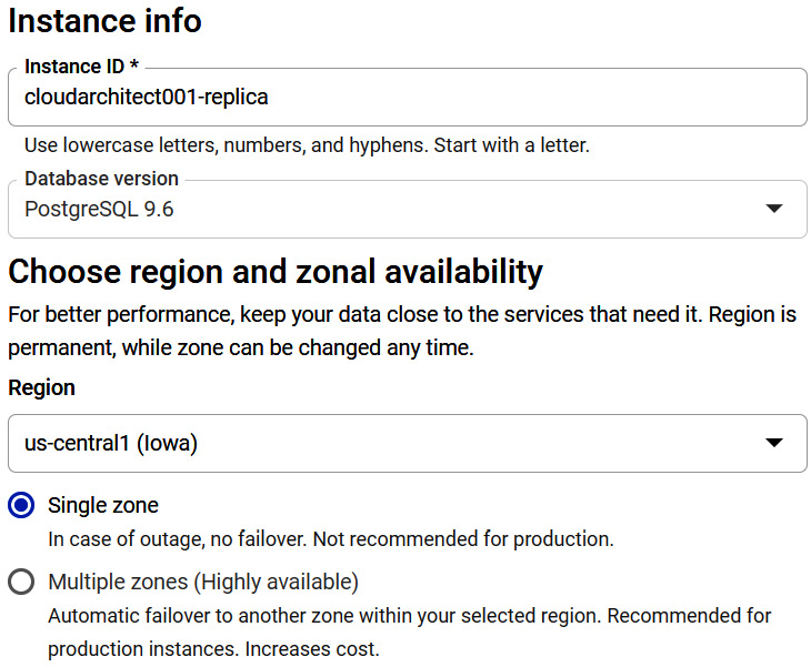
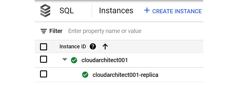
Figure 11.34 – Viewing the read replica
In this section, we looked at read replicas and the various options available. In the next section, we will look at failover replicas.
High availability
I am sure we are all familiar with the term HA. The purpose of this is, of course, to reduce the downtime of a service and in terms of Cloud SQL, to reduce the downtime when a zone or instance becomes unavailable. Public clouds are not immune to downtime and zonal outages can occur, as well as instances becoming corrupted. By enabling HA, our data continues to be available to client applications. As we discussed in the previous section, when deploying a new Cloud SQL instance, we can select a multiple zone configuration to enable HA, which means two separate instances are created within the same region but in different zones. The first instance is configured as the primary, while the second is used as a standby. Through synchronous replication to each zones persistent disk, all writes that are made to the primary instance will be replicated to the disks in both zones before the transaction is confirmed as completed. In the event of a zone or instance failure, the persistent disk is attached to the standby instance, which will then become the new primary instance. Users are then routed to this new primary instance. This process is described as a failover. It is important to note that this configuration will remain even when the original primary instance comes back online. This is because once the original primary instance becomes available once more, it is destroyed, recreated, and becomes the new standby instance. If there is a need to have the primary instance in the original zone, then a failback can be performed. This process is the same as a failover but is where we are making the decision.
Please note that until Q1 2021, legacy MySQL had an HA option for using failover replicas. This is no longer available from Cloud Console.
Backup and recovery
We mentioned backup and recovery previously when we created a new instance. We can create a backup schedule and trigger an on-demand backup from our console or command line whenever required. If we want to edit our instance, we have to check the backup schedule that we have configured or change the backup time if necessary:
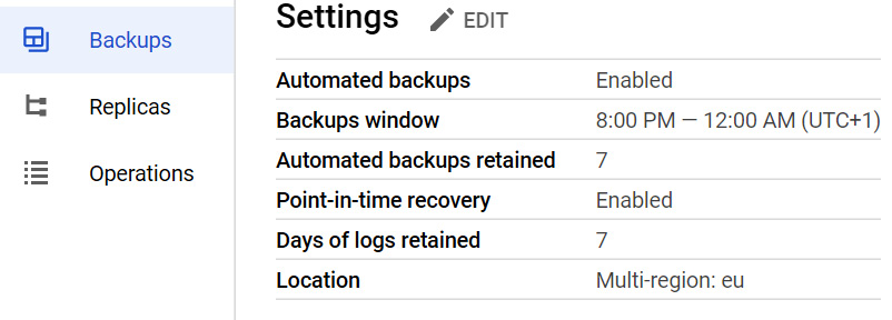
Figure 11.35 – Editing the backup schedule
Backups are a way to restore our data from a certain time in the event of corruption or data loss. Cloud SQL gives us the option to restore data for the original instance or a different instance. Both methods will overwrite all of the current data on the target instance.
Let's look at how we can restore from the console:
- From our MySQL deployment, we can click on the BACKUPS tab and then scroll to the bottom of the page for the specific backup we would like to restore:

Figure 11.36 – Selecting a backup
- If we don't have any replicas or we have deleted them, then we can proceed. You will notice that we can restore directly back to the source instance or select another instance:
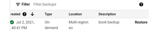
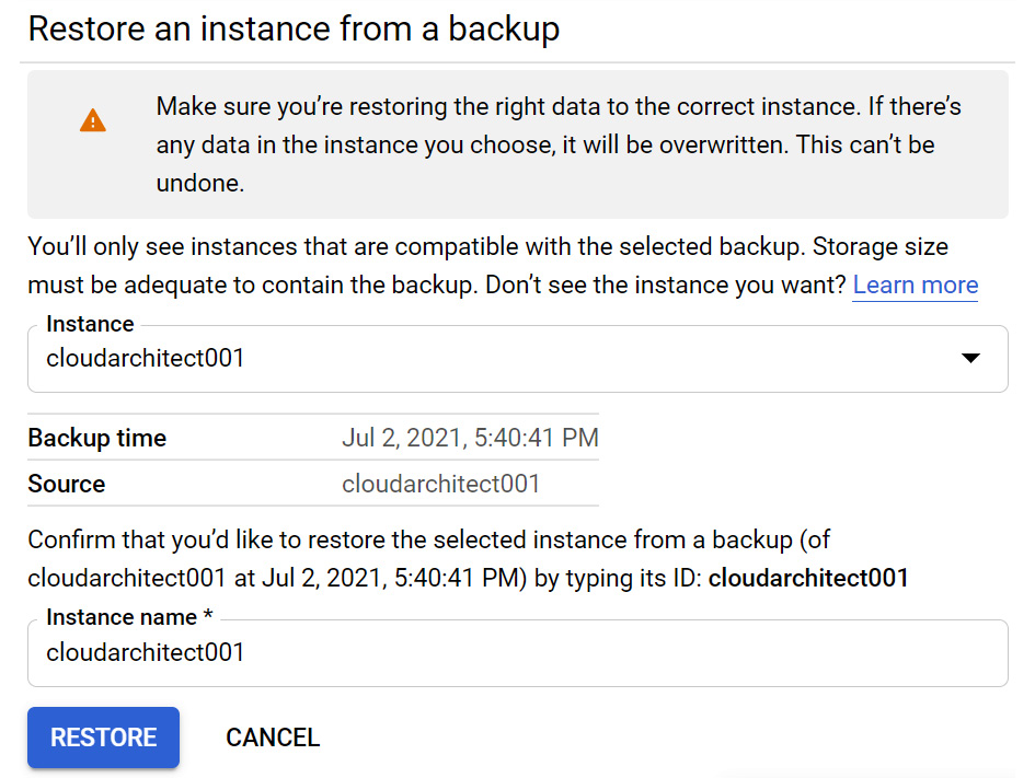
Figure 11.37 – Restoring a backup
In the next section, we will look at how to migrate data.
Database migration service
GCP now offers a service that allows us to easily migrate databases to Cloud SQL from on-premises, Compute Engine, or even other clouds. In essence, this is a lift and shift for MySQL and PostgreSQL workloads in Cloud SQL. This is an ideal first step for organizations looking to move existing services into a public cloud as it means less infrastructure to manage and also enjoying the HA, DR, and performance benefits of Google Cloud.
Instance cloning
We previously mentioned that we can clone our instances. This will create a copy of our source instance, but it will be completely independent. This does not mean that we have a cluster or read-only replica in place. Once the cloning is complete, any changes to the source instance will not be reflected in the new cloned instance and vice versa. Instance IP addresses and replicas are not copied to the new cloned instance and must be configured again on the cloned instance. Similarly, any backups that are taken from the source instance are not replicated to the cloned instance.
This can be done from our GCP Console or by using our gcloud command-line tool:
- Let's look at the syntax that we would use to perform this:
gcloud sql instances clone <instance source name> <target instance name>
Here, <instance source name> is the name of the instance you wish to clone, while <target instance name> is the name you wish to assign to the cloned instance.
- Let's look at how to clone our cloudarchitect001 instance:
gcloud sql instances clone cloudarchitect001 cloudarchitect001cloned
We will call the cloned instance cloudarchitect001cloned.
IAM
Access to Google Cloud SQL is secured with IAM. Let's have a look at the list of predefined roles and their details:
- Owner: Has full access and control over all GCP resources
- Editor: Has read-write access to all SQL resources
- Viewer: Has read-only access to all Google Cloud resources, including Cloud SQL resources
- Cloud SQL Admin: Has full control of all Cloud SQL resources
- Cloud SQL Editor: Has rights to manage specific instances; can't see or modify permissions or modify users for SSL certificates; cannot import data or restore from a backup nor clone, delete, or promote instances; and cannot stop or start replicas or delete databases, replicas, or backups
- Cloud SQL Viewer: Has read-only rights to all Cloud SQL resources
- Cloud SQL Client: Has access to cloud SQL instances from App Engine and Cloud SQL Proxy
- Cloud SQL Instance User: Allows access to a Cloud SQL resource
Quotas and limits
Google Cloud SQL comes with predefined quotas. These default quotas can be changed via the Navigation menu, under the IAM & Admin | Quotas section. From this menu, we can review the current quotas and request an increase to these limits. We recommend that you familiarize yourself with the limits for each service as this can have an impact on your scalability. For Cloud SQL, we should be aware of some important limits.
Exam Tip
MySQL (second generation) and PostgreSQL have a storage limit of 10 TB.
Other limits to be aware of include the following:
Pricing
Pricing for Cloud SQL is based on CPU and memory pricing, storage and networking pricing, and instance pricing.
For CPU and memory, it is dependent on location, the number of CPUs, and the amount of memory you plan to use. Read replicas are charged at the same rate as standalone instances.
For storage and networking, it is dependent on location, per GB of storage used per month, and the amount of egress networking from Cloud SQL.
Instance pricing is also dependent on where the instance is located and the shared-core machine type.
Summary
In this blog, we covered the storage options available to us by looking at which ones were most appropriate for common requirements. We also learned about Google Cloud Storage, Cloud Firestore, and Cloud SQL.
With Google Cloud Storage, we looked at use cases, storage classes, and some main features of the service. We also covered some considerations to bear in mind when transferring data. It's clear that Cloud Storage offers a lot of flexibility, but when we need to store more structured data, we need to look at alternatives.
With Cloud Datastore, we learned that this service is a NoSQL database and is ideal for your situation, should your application rely on highly available and structured data. Also, Cloud Datastore can scale from zero up to terabytes of data with ease and is ideal for ACID transactions. We also learned that it offers eventual or strong consistency; however, if we have different requirements and a need for a relational database that has full SQL support for Online Transaction Processing (OLTP), then we should consider Cloud SQL.
For Cloud SQL, we learned that we have different offerings – MySQL, SQL Server, and PostgreSQL. We reviewed how to create and manage our instances, how to create replicas, and how to restore our instances.
In the next article, we will continue looking at GCP storage options by covering Cloud Spanner and Bigtable.
Further reading
Read the following articles for more information on the topics that were covered in this article:
- Cloud Storage: https://cloud.google.com/storage/docs/
- Cloud Datastore: https://cloud.google.com/datastore/docs/
- Cloud SQL: https://cloud.google.com/sql/docs/
- Cloud SQL pricing: https://cloud.google.com/sql/pricing
- Importing data into Cloud SQL: https://cloud.google.com/sql/docs/mysql/import-export/importing
- Exporting data from Cloud SQL: https://cloud.google.com/sql/docs/mysql/import-export/exporting