 In the previous article we introduced Essbase and Oracle OLAP, and showed how they both offer effective solutions for OLAP. The similarities between the products arise from a shared goal to provide business users with the technology they need to perform ad hoc analysis and to report on centralized data stored on a server. The differences between the two products stem primarily from who is responsible for (or "owns") the OLAP solution, how it is implemented and accessed, and where the OLAP data is stored.
Essbase is owned and managed, generally speaking, by line-of-business users in partnership with the IT group. Essbase uses a multidimensional database stored on disk and in RAM. In contrast, the organization's IT group typically owns Oracle OLAP, in partnership with line-of-business users. Oracle OLAP is a natural part of the Oracle Database, which means it can take advantage of other database features (such as security and access to data via SQL) and other options (such as Oracle Real Application Clusters). The similarities and differences are reflected in how each product implements OLAP concepts.
In this blog article, we introduce common OLAP concepts - such as multidimensionality, calculations, and ad hoc analysis - and show how the concepts are implemented in Essbase and Oracle OLAP. In subsequent sections, we will build on this foundation, explaining product-specific implementations in more detail. We conclude this blog with histories of Oracle OLAP and Essbase. The business problem each product was designed to solve and the evolution of each product help to explain the differences between the two products.
Common OLAP Themes
OLAP relies on a basic set of concepts. These concepts are shared between Oracle OLAP and Essbase. For the purposes of this blog, we have organized the concepts into the following logical groupings:
- Multidimensional view of information The concepts of a cube, dimensions, members, hierarchies, levels, attributes, measures, and aggregation
- From data source to multidimensional data Data-related concepts such as transformation from transactional data sources to multidimensional cubes, dense and sparse cubes, partitions, slowly changing dimensions, user access to data, and write-back functionality
- New results from existing data Advanced aggregation operators and calculated measures that are derived from data stored in multidimensional cubes
- Ad hoc analysis Having a conversation with the data by using drill paths, pivoting dimensions, and manipulating data subsets
The following sections describe each group of concepts, including how Essbase and Oracle OLAP implement them. The goal here is to map the conceptual terms to particular features within each product so that you can begin to build up some product-specific vocabulary. Note that product-specific features are only briefly introduced here.
Multidimensional View of Information
We defined the term OLAP in the this blog note, but you may also encounter another term that is used interchangeably: multidimensional analysis. Multidimensional means nothing more than thinking about a topic from more than one perspective. For example, consider your answers to the following questions:
- Where are you currently located?
- What day of the week is it?
- What are you doing right now?
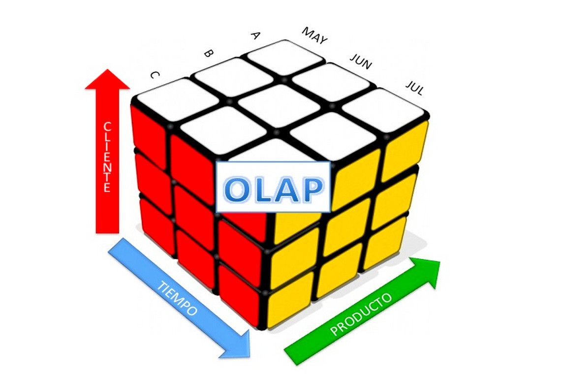
You just performed your first piece of multidimensional analysis - analyzing location by time and task. In this example, location, time, and task are dimensions. Your specific answers to these questions - let's say head office, Monday, and reading - are members within the dimensions. In a multidimensional analysis, the dimensions can be thought of as forming the edges of a cube, with the names of the dimension members defining where you are on each edge.
A fundamental principle of OLAP systems is to optimize how data is stored so that it may be accessed as quickly as possible by the end user to support ad hoc analysis. Unlike transactional systems built with relational databases, or even data warehouses built on relational databases, OLAP systems provide highly optimized structures to store and aggregate data. The purpose of these systems is to precalculate measures that could possibly be used as part of the analysis. The precalculation happens when loading the data. A lot of the generic "overhead" used to store data in a relational database is omitted from OLAP cubes. The following discussion summarizes the concepts used to precalculate and efficiently store data so that access to the data is blazingly fast.
Cubes
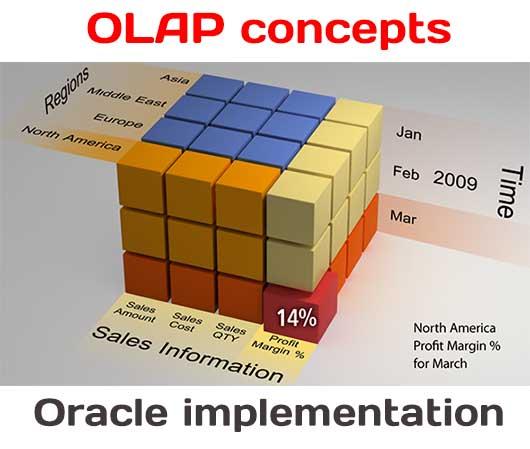
We introduced the concept of a cube in this article. To recap, Figure 1 shows three dimensions, one on each axis of the cube. The intersection of members from each dimension has the potential to hold a value. The values represent a measure, which is sales in this case.
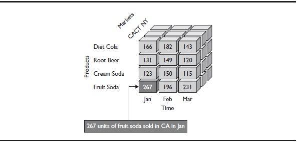
Figure 1. Dimensions represented in an OLAP cube
Fundamentally, Essbase and Oracle OLAP implement the concept of a multidimensional cube differently. Although Essbase applications can be made up of a series of interconnected cubes, they often store all data in a single cube that represents all possible combinations of all dimensions. Using the term cube in this context is a bit of a stretch, and sometimes the term hypercube is used to suggest the higher dimensionality. An Essbase cube is more accurately referred to as an Essbase multidimensional database, where the data is stored in a multidimensional structure rather than a relational structure, though the terms are often used interchangeably.
In this blog's discussion of generic OLAP concepts, we will continue to use the term cube to describe an Essbase database.
In Oracle OLAP, data is stored in cubes of varying dimensionality. Specifically, the data and the type of analysis required determine the number of dimensions represented in any given cube. For example, sales data may be broken down by four dimensions: region, time, channel, and product, but budgetary data may be broken down only by channel or region. With Oracle OLAP, you can specify the dimensions for each of the two cubes independently. A single cube is often loaded from a central fact table and the associated dimension tables. These cubes are presented as a star schema, and can be used as cube-organized materialized views in the larger relational database, which will be discussed in more detail in other articles of my blog.
From a practical standpoint, the functionality that is exposed to the end user from either Essbase or Oracle OLAP is very similar. End users can interact with their data in an easy-to-understand, intuitive fashion. How the application is built and maintained relates to the core differences of the two products.
Dimensions, Hierarchies, and Members
A dimension is a collection of items that share some attribute or characteristic. You define dimensions for those attributes or characteristics that you want to report or analyze. Dimensions contain members such as January or February, which are often organized into one or more hierarchies.
The concept of a hierarchy is intuitive. Hierarchies are how human beings like to think of and categorize concepts. For example, if you have ever written an essay in school, you organized the information in a hierarchy.
1 Animals a.
Dogs
| I | Labrador |
| II | Shepherd |
| III | Terrier |
A typical dimension consists of one or more members, each of which may contain one or more hierarchies of members. Figure 2 shows partial dimension hierarchies for Time, Products, and Markets.
The relationships between members within a dimension define the dimension hierarchy. OLAP systems often use a genealogical model to explain the relationships among members, so we can talk about members having children, parents, siblings, ancestors, and descendants. In Figure 2, Sodas has two children (Fruit Soda and Cream Soda), one parent (Products), and at least one sibling (Colas).
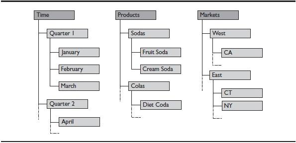
Figure 2. Dimension hierarchy
Another way to talk about a member is by its location, or level, within a hierarchy. In Figure 2, the Time dimension has three levels: time (which corresponds to the year), quarters, and months. Members with no children are called base-level members or leaf members. In this Time dimension, the base-level members are the 12 months of the year.
When a hierarchy contains at least one base-level member at a different level than the other base-level members, it is called a ragged hierarchy. Ragged hierarchies are very common in OLAP systems, as they typically explain the complexity in the real world. For example, in Figure 3, the sales for a company are broken down by region of the country and then state for the United States, but only by a few provinces for Canada, and simply by country for Mexico. This type of hierarchy reflects that business people tend to think about the business in groups that are of a similar size. In the example in Figure 3, the company has sales that are approximately equal across the regions in the United States, within the selected provinces in Canada, and for the entire country of Mexico.
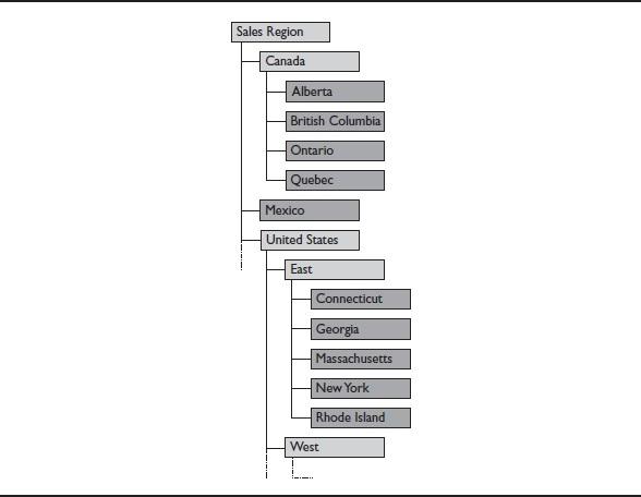
Figure 3. A ragged hierarchy with leaf nodes highlighted
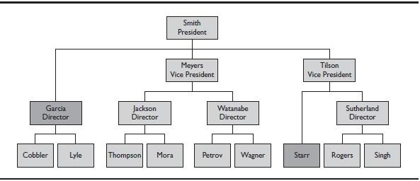
Figure 4. Skip-level hierarchy with skip-through nodes highlighted
When a hierarchy has at least one member whose parent is more than one level above it, the hierarchy is referred to as a skip-level hierarchy. For example, in Figure 4, the president, Smith, has vice presidents as well as a director reporting to him. The director, Garcia, skips through the vice president level. Another skip-level occurs in Tilson's reporting structure, where Tilson has a director (Sutherland) as well as a regular employee (Starr) reporting to her. Starr skips through the director level. Again, multidimensional systems make it easy to represent the real world in an intuitive manner.
Robust OLAP systems, including Oracle OLAP and Essbase, support ragged hierarchies and skip-level hierarchies.
NOTEThe homogenous use of a single dimension representing multiple levels is sometimes confusing to DBAs who are used to relational database concepts. Columns in a relational table can store only one type of item, such as a month or a year; they cannot store both types. In an OLAP application, to select Just months, you simply ask for times at the month level.
Oracle OLAP and Essbase implement dimensions, hierarchies, and members in similar ways. They use the language of genealogy to describe member relationships. Both products also implement the concept of levels, but in different ways. In Oracle OLAP, you define and label levels in a hierarchy. You can also have value-based hierarchies, where the parent-child structure is in place, but specific levels are not identified - just the depth from the top. Essbase automatically identifies levels in two ways: levels and generations. Levels are numbered from bottom to top, where level 0 is a leaf member (a member with no children), level 1 is its parent, and so forth up the hierarchy. Generations are numbered from top to bottom, where generation 1 is the root of the dimension, generation 2 is all its children, and so forth down the hierarchies. Essbase also allows user-defined level names. In all cases, you can use levels to map source data to locations within dimension hierarchies.
Attributes
An inherent value of an OLAP system is the ability for business users to analyze data in a way that makes sense to them. We do this every day when we make a decision based on a variety of environmental and personal points of view. To that end, OLAP models have evolved to provide the ability to view data in a variety of ways.
One way to provide alternate views of the data is through user-defined attributes or groupings. An attribute is a tag or property assigned to a member. For example, you might tag some Market members as "Major Market," so that an end user can easily find and present all of the major markets in a report.
Oracle OLAP and Essbase approach user-defined attributes in the same way - that is, as tags assigned to members. Users can create as many different attribute tags as they need to suit their purposes. Attributes can be assigned to any dimension, and a member can have multiple attributes associated with it. There are no calculations inherent in attributes, but attributes can be used within calculations. In addition to user-defined attributes, Essbase also has a dimension type called an attribute dimension, which provides a way to create alternate hierarchies based on a characteristic of the members.
Alternate Hierarchies
Another way to get alternate views of the data is to define more than one hierarchy for a dimension. Alternate hierarchies provide different ways to aggregate a dimension. For example, a Customer dimension may have a geographic hierarchy and a managerial hierarchy, as shown in Figure 5. If analysis is typically performed using one of these hierarchies (but not both at the same time!), this is best done with two hierarchies of the same dimension. OLAP products ensure that data is not counted more than once when using alternate hierarchies.
The products differ in their implementation of alternate hierarchies. In Oracle OLAP, each dimension has a current hierarchy that defines the current drill path
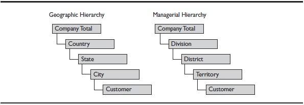
Figure 5. Multiple hierarchies for a Customer dimension
for the dimension. Users can select a hierarchy to use as their current hierarchy. Because users are working with only one hierarchy of a dimension at a time, there is little risk in counting the data multiple times. In Essbase, alternate hierarchies can be defined in two ways: by creating attribute dimensions and by creating hierarchies that contain shared members (pointers to members in the primary hierarchy). Users can drill through to different hierarchies as easily as drilling down from one level to the next. We define and discuss drill paths in the "Ad Hoc Analysis: Having a Conversation with Your Data" section later in this article.
Unique Versus Duplicate Members
A discussion about alternate hierarchies generally leads to another discussion - one concerning the concepts of unique and duplicate members. A duplicate member occurs when you use the same member name for more than one member.
For example, consider an OLAP system for a shipping company that has a dimension for Origin and another dimension for Destination. A customer in San Francisco could both send and receive packages from that location, which means that the customer would legitimately need to belong to both dimensions. Although the company could create unique names, a more elegant solution from the user perspective would be to allow the customer to exist in both dimensions, and use the context of the member within the hierarchy to provide the uniqueness.
This approach to creating uniqueness is similar to that used in object-oriented programming, where the larger class defines the unique attributes of the member.
Essbase and Oracle OLAP support duplicate members. In Essbase, member names are assumed to be unique unless you enable support for duplicate members.
Duplicate members are made unique by prefixing the member name with its ancestors, up to and including the dimension name. Oracle OLAP, on the other hand, has no unified list of dimension values across all dimensions, so duplicate members across dimensions are not an issue. Oracle OLAP offers support for duplicate members within a dimension using surrogate keys. Support for surrogate keys is on by default. In Oracle OLAP, level names in a hierarchy are user-defined. Oracle OLAP makes the member name unique by prefixing the member name with the level name.
NOTE
In Essbase, working with a model that contains duplicates is more complex from a reporting perspective. In this article, assume that all examples are created using unique member names only.
Dimensions, hierarchies, members, levels, and attributes form the structure of a cube. The data comes from measures.
Measures and Values
Measures represent business data that is important for analysis, such as sales and cost of goods sold. Measure values are the data that fills the intersections in a cube. To be meaningful, a value must be defined in terms of all dimensions in the cube (hence the term multidimensional analysis). For example, in Figure 1, we determine the meaning of the highlighted sales value of 267 by examining the dimension members that form the intersection at that value, and so we understand that 267 units of soda were sold in California in January.
TIP
For those with a relational database data warehouse background, a measure is synonymous with a fact in a fact table. When a relational database provides the source data, unique key columns are often the dimensions and fact columns are often the measures.
Stored measures are values saved in the cube. Calculated measures are values derived from calculations based on stored measures and/or other calculated measures.
Oracle OLAP and Essbase have some key similarities in how they implement
measures. Both products allow for stored measures and calculated measures (though Essbase uses the terms stored values and calculated values instead). In each case, decisions must be made about the level of detail to include in the cube; for example, it may be more appropriate to provide summary-level data in a cube rather than detailed data.
The products also have differences in how measures are handled:
- With Oracle OLAP, you create multiple cubes of varying dimensionality, which means that understanding the context of a measure is straightforward. Measures are organized by their dimensions and typically include a Time dimension. In contrast, Essbase includes all dimensions in its multidimensional database, so querying and understanding the meaning of an individual measure can be more complex, because you need to think across more dimensions.
- Oracle OLAP has no internal representation of a "measures dimension" per se, and no hierarchy of measures, whereas Essbase has a dimension type for measures called What makes an accounts dimension special is that Essbase calculates the accounts dimension first. Other than that, it behaves exactly like any other dimension stored in the cube.
- With Essbase, any dimension can have calculated values, whereas with Oracle OLAP, calculated measures can be defined, but calculated values of other dimensions require special techniques called In Oracle OLAP 11g Release 1 and earlier, this is done in OLAP Worksheet via the OLAP Data Manipulation Language (DML). Models can be defined for any dimension by database administrators.
Aggregation
OLAP systems leverage the concept of hierarchies for calculation purposes, providing default calculations simply by aggregating the values of the members up the hierarchy. Take the Time dimension in Figure 2, for example. Time has a value that represents the total of the values for each of the four quarters in the year. The quarter members get their value from the summation of the months within the quarter. This speeds the access to information and makes it easy for the OLAP system to find the values and present them to end users.
Both Essbase and Oracle OLAP implement the concept of aggregation. Aggregation, by default, is addition. You can turn off aggregation or change the operation from addition to some other operation. We discuss aggregation operators, as well as other ways to perform calculations, in more detail in the "New Results from Existing Data" section later in this blog. With both Oracle OLAP and Essbase, aggregations can occur either in some batch process or on the fly as a user is querying the cube.
From Data Source to Multidimensional Data
In the previous section, we talked about measures as the data in the cube. All OLAP systems pull data into cubes from one or more data sources. An important part of both OLAP engines is how the data will be stored to optimize efficient access to respond to end-user queries. In this section, we discuss concepts related to data, including data sources, dense and sparse cubes, partitions, security of the data, and write-back to the cube.
Data Sources
A company's source data often comes from transactional systems, such as point-of- sale or customer relationship management (CRM) applications. To perform an OLAP analysis, source data needs to be made available to the OLAP engine. We use the phrase "made available" very deliberately, because depending on the type of OLAP implementation, data may or may not need to be moved into the OLAP engine.
Data Sources and OLAP Types .An OLAP engine stores and accesses data differently, depending on the type of OLAP implementation. The three main types of OLAP are multidimensional OLAP (MOLAP), relational OLAP (ROLAP), and hybrid OLAP (HOLAP), which store data as follows:
- With MOLAP, the engine stores data - often aggregated data - in a multidimensional structure.
- With ROLAP, data is stored in a relational source, and the OLAP engine generates dynamic SQL to extract the data for analytical processing at query time.
- With HOLAP, the engine stores some data in the OLAP engine and some data in a relational data source. Depending on the level of detail required for the query or analysis, the data may need to be accessed from one or both locations. For example, if you have a model that analyzes sales patterns across the United States, you might store data down to the city level in the OLAP structure, but leave granular data like zip (postal) codes in the relational structure. The decision to store data in one location or another is most often a factor of processing efficiency and query performance requirements.
Relational Database Schemas.When mapping a relational data source to a cube, OLAP products make use of the relational source's star or snowflake schema as a way to define dimensions and hierarchies.
As illustrated in Figure 6, a star dimensional model uses fact tables and a set of smaller dimension tables. The star dimensional model is a flat model that allows for
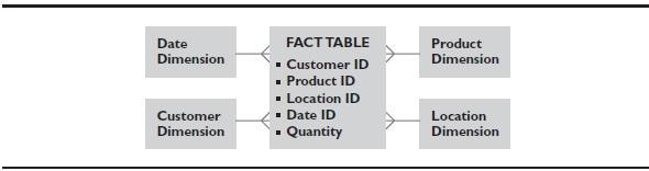
Figure 6. Star model with one fact table and smaller dimension tables
easier user access than third normal form. Dimension tables act much like foreign key tables or reference tables in an online transactional processing (OLTP) system. Fact tables have key values that relate to the dimension tables and fact columns, such as quantity.
A snowflake model is an extension of a star dimensional model, as illustrated in Figure 7. It normalizes and aggregates the dimensions in a star dimensional model. This has the effect of creating more tables and requires more SQL joins.
Both Oracle OLAP and Essbase have administrative applications that can read a star or snowflake schema and present the tables for selection in an OLAP cube.
Multidimensional Storage and Access
Speed-of-thought response time to queries is a hallmark of OLAP. The way OLAP engines store and retrieve data is necessarily different from a traditional, relational database-based, data warehouse approach. Before we visit OLAP solutions, let's explore how traditional data warehouses typically access data
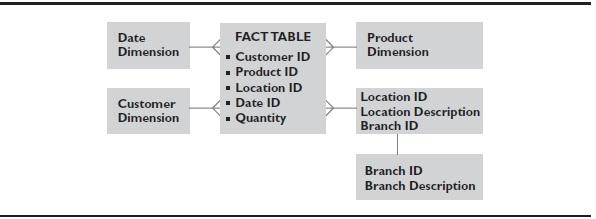
Figure 7. Snowflake model
Traditional Data Warehouse Approach - Bitmapped Indexes Bitmapped indexes are important for data warehouses. Bitmapped indexes logically map each row with each distinct data value. Bitmapped indexes are generally chosen over a B-tree data structure for low-cardinality columns. Low cardinality is determined by dividing the number of distinct column values by the total number of rows. If the result is below 5 percent, the column has low cardinality. For example, a one million row table might have a State column that has only 50 distinct values. In this case, the State column has low cardinality, since 50 divided by 1 million is less than 5 percent.
A properly designed bitmapped index is approximately ten times smaller than a B-tree data structure. As these indexes must be stored as structures in the data warehouse and consume disk space storage, there is a constant tension between how much indexing is needed versus how much space is to be consumed and taken away from the data. Because of its much smaller size, a bitmapped index is ideal for traditional data warehouses.
An OLAP Approach - Arrays At its most basic level, OLAP products store multidimensional data in arrays. Arrays provide a way of organizing OLAP data. Data is stored very efficiently, since the keys (dimension values) are kept separate from the data in the cube. OLAP dimensions are analogous to an array's subscripts. The dimensions serve as a sort of index to the array, and they provide fast access to the data. Data in arrays can be located with simple arithmetic.
In Oracle OLAP, the implementation of the array-based storage concept is more sophisticated than simple arithmetic, especially with respect to sparse data sets. For example, aggregate compression delivers very sophisticated algorithms for storing and retrieving data optimally. Oracle OLAP automatically manages retrieving data from disk when required and caching the data in memory as appropriate.
Essbase has two approaches to storing data: block storage and aggregate storage. For block storage, data is stored in an array. For aggregate storage, data is stored in tablespace - similar to a large array - as a collection of cells. We discuss the two types of storage models in more detail in other blog notes.
Essbase handles data and requests for data using two primary structures: indexes and a data storage mechanism (array or cell). Whenever a data value is queried, loaded, or calculated, Essbase brings the specific data storage file into memory. To find the proper data, Essbase uses an index. All data values in the model are indexed. Essbase holds this index in RAM (in many cases), and each request first goes to the index to find the data location. Once identified, Essbase brings that data into RAM to perform the requested action. Both the data index and data files are compressed while on disk, and to a lesser degree, in RAM. The nature of the compression varies depending on the type of numeric data stored in the structure.
Dense and Sparse Cubes
Density is a ratio of the total number of cells in an OLAP cube that are populated with a value versus the total number of possible cells in the cube. The closer this ratio is to 1, the denser the OLAP cube; the further away from 1, the sparser the cube. For example, consider a cube that contains sales data by time by products by markets. If most of the products are sold in most of the markets over the year, then most of the cells contain data, and the cube is dense. If the opposite is true - most products are not sold in most markets - many of the cells are empty, and the cube is sparse.
Sparse cubes take more space than necessary to store because space is reserved for every cell, whether or not it has data in it. They may also take longer than necessary to calculate, because null data cells are considered for calculation along with values. OLAP systems use different approaches to address sparsity of data.
In Essbase, most cubes are inherently sparse because they contain all dimensions. Essbase handles sparsity in two ways, depending on which type of data storage is in use: block or aggregate. We will talk more about storage types later. For the moment, it is sufficient to know that, for block storage databases, Essbase requires that the administrator tag dimensions as dense or sparse at the outline level, so that it knows how to store the data. For example, a Time dimension is usually dense, while a Product dimension is often sparse. In aggregate storage databases, Essbase does not require the dense/sparse tag; it handles sparsity at the storage level.
In Oracle OLAP, the administrator defines a dimension as sparse. For all sparse dimensions, Oracle OLAP defines a special type of dimension called a composite. The composite holds only the combinations of the sparse dimensions that actually contain data. This composite is maintained automatically by Oracle OLAP and is integrated with its advanced compression algorithms for handling aggregate data.
Partitions
Whenever a database handles volumes of data, the concept of data partitioning across multiple data storage becomes important. In a data warehouse environment, for example, partitioning allows huge tables to be broken up into a series of smaller tables with faster access, but the SQL application can query the series of smaller tables as if it were one big table. With partitioning, a data warehouse can expand to many hundreds of terabytes, while ensuring that results are returned in a reasonable amount of time. A partitioned architecture also enables you to drop a partition, which takes less than a second. If you do not partition, deleting old data could take a long time.
OLAP cubes can also benefit from partitioning data. By partitioning your data, you can break your data into more manageable chunks, but you are able to hide the complexity of this strategy from the application and end user. For example, you could partition a Time dimension so that historical data (say, older than five years) is kept in a separate partition, allowing faster access to data from more recent years. When implemented effectively, partitions help to ensure fast, reliable, and concurrent access to OLAP data.
Oracle OLAP and Essbase both offer partitioning strategies. Oracle OLAP allows you to define a dimension as a partitioning dimension. Generally, you identify a level (such as year) of the partitioning dimension, although more complex designs are possible. Cubes are physically separated into individual partitions for each year, but the partitioning scheme is transparent to applications that query or write to a cube. At query time, partition pruning occurs - meaning if you partition by year and ask for data for a single year, only one partition is accessed for the data. Partitions can be added and removed easily.
In Essbase, you can think of a partition as a region of a cube that is shared with another cube. Partitions come in three types:
- Replicated partitions allow you to store data in different cubes and copy shared data from one cube to another.
- Transparent partitions enable users to navigate seamless from locally stored data to remotely stored data.
- Linked partitions provide a means of linking a cell in a cube to a different cube with potentially different dimensionality.
We discuss Essbase partitioning strategies in next article of my blog.
Slowly Changing Dimensions
Slowly changing dimensions are dimensions that change over time - sometimes a little, but sometimes (perhaps because of an acquisition) a lot. For example, consider a cube that tracks personnel data. The dimension that tracks employee names is a slowly changing dimension because it is possible for the names, in particular the surnames, to change. While you could simply overwrite the data, it may be important to track the changes.
Handling slowly changing data effectively is critical in any database. Data warehousing theory proposes methods for managing changing data that we can also apply to OLAP cubes:
- Type 1: Replace the value
- Type 2: Add a record with an effective start date and effective end date
- Type 3: Store the old value
- Type 6: A combination of Types 1,2, and 3
Because slowly changing dimensions are so important, let's take some time to understand how each type works before we look at how Oracle OLAP and Essbase implement this concept. For this discussion, we will use the following example: Mary Smith marries Bob Jones and decides to change her name to Mary Jones.
Type 1 In Type 1, the column or attribute value is simply overwritten and the previous value is lost. In our example, a Type 1 methodology would just change the member dimension to update the last name from Smith to Jones. The fact that Mary was once Mary Smith is lost. For example, this data:
| Key | First Name | Last Name |
| 12345 | Mary | Smith |
becomes this data:
| Key | First Name | Last Name |
| 12345 | Mary | Jones |
Type 2 In Type 2, an additional record is created, as well as fields for the effective start date and the effective end date. In our example, a Type 2 methodology would add a new record for Mary Jones with the effective start date of today. The old record would have the effective end date updated with today's date. The fact that Mary was once Mary Smith is not lost.
| Key | First Name | Last Name | Eff_Start | Eff_End |
| 12345 | Mary | Smith | 1/18/1960 | 3/14/2006 |
| 45678 | Mary | Jones | 3/14/2006 |
Type 3 In Type 3, an attribute is added to the record. In our example, a Type 3 change would add fields to the record to contain the old name. The old last name field would be set to Smith, and the current last name field would be changed to Jones.
| Key | First Name | Last Name | Prior First Name | Prior Last Name |
| 12345 | Mary | Smith | Mary | Jones |
Type 6 Type 6 combines Types 1,2, and 3. Expanding on our example, let's say that Mary Smith was born on 1/18/1960. Mary Smith marries Bob Jones and
becomes Mary Jones on 3/14/2003. On 7/24/2005, Mary Jones divorces Bob Jones. On 9/17/2005, Mary Jones marries Mark Davis and chooses to take his last name.
| Current | Current | Historical | Historical | ||||
| First Name | Last Name | First Name | Last Name | Eff_Start | Eff_End | |
| 12345 | Mary | Smith | Mary | Smith | 1/18/1960 |
| Current | Current | Historical | Historical | ||||
| Key | First Name | Last Name | First Name | Last Name |
| Eff_End | |
| 12345 | Mary | Jones | Mary | Smith | 1/18/1960 | 3/14/2003 | |
| 45678 | Mary | Jones | Mary | Smith | 3/14/2003 |
| Current | Current | Historical | Historical | ||||
| Key | First Name | Last Name | First Name | Last Name | Eff_Start | Eff_End | |
| 12345 | Mary | Davis | Mary |
| 1/18/1960 | 3/14/2003 | |
| 45678 | Mary | Davis | Mary | Jones | 3/14/2003 | 7/24/2005 | |
| 56789 | Mary | Davis | Mary | Jones | 9/17/2005 |
This method gives us the most flexibility, but at the highest cost in terms of space and maintenance.
Oracle OLAP and Essbase Implementation Both Oracle OLAP and Essbase support slowly changing dimensions. In Oracle OLAP, you can model slowly changing dimensions using attributes and measures. For example, to model the preceding example, you would simply map the key column to the dimension member. Type 1 will be handled automatically - when the dimension is maintained, the name will change. For Type 2 and Type 3, simply add attributes or measures for the Eff_Start and Eff_End and Prior First Name and Prior Last Name to allow the user to choose which dimension members to use for selection or display purposes. For Type 6, you can add attributes and measures for the historical names as well.
In Essbase, you can model slowly changing dimensions using user-defined attributes, aliases, alternate hierarchies created with shared members, or varying attributes. For example, to model the preceding example in a Type 1 scenario, you would simply change the name of the Mary Smith member to Mary Jones. For Type 3, you could use an alias, so that the member name remains unchanged, but you could use the new name for query and display purposes. If you need to track when the surname changed, as in a Type 2 scenario, a user-defined attribute or varying attribute may be more appropriate. Alternatively, if you are mapping a Type 2 or Type 6 approach directly from the relational source to an Essbase cube, you can load the columns into Essbase as usual, and then vary attributes across time on the Historical Last Name.
Security and User Access
The security of the data in OLAP systems is critical. Some organizations have all-or- nothing security procedures, meaning that you can either see the data or you cannot see the data. More often, various groups of users need access to specific portions of OLAP cubes. For example, maybe the Eastern region manager should have access to only the data for the Eastern region and all of the customers in the Eastern region. A robust OLAP system offers the ability to set user access for the cube, as well as at various levels in the cube, including dimensions and measures.
Oracle OLAP leverages Oracle Database user accounts, passwords, and security measures to protect data, using commands such as GRANT to control access to cubes, just like any other database object such as tables. In addition to this overall security, object security lets you grant and revoke access to dimensional objects using SQL. For data security, Analytic Workspace Manager (AWM) allows you to control access to sections of a cube at the cellular level, in a fashion similar to virtual private databases (VPDs), typically for each dimension.
Similar to Oracle OLAP, Essbase supports detailed user and group security. Essbase provides general security for cube access and administrative roles (such as the ability to provision users). Additionally, Essbase allows for a series of optional security levels on objects as well as data and metadata. From a data and metadata perspective, Essbase supports security down to the cell level.
Write-Back to the Cube to Build Scenarios
Write-back provides end users with the ability to change the values in the cube. End users can try out various scenarios (called scenario playing) by posing "what-if" type questions. For example, a business user might want to see what would happen if sales for a product or set of products increased by 5 percent. Many modeling and planning applications are based on scenario playing. When OLAP systems support scenario playing, system administrators assign write-back permission to authorized end users.
Essbase and Oracle OLAP support scenario playing and write-back via front-end applications. Essbase has write-back built in as a basic feature. Oracle OLAP provides the capability via the BI Spreadsheet Add-in, through the OLAP DML, or by using SQL to change the original source tables. For both products, administrators grant write access using the standard user access and security mechanisms for each product.
New Results from Existing Data
At the heart of an OLAP solution is the ability to perform quick and often complex calculations. In addition to the aggregation, OLAP engines contain hundreds of prepackaged calculation functions, ranging from a simple average function to the more complex allocation, return on investment (ROI), and trend functions. Many OLAP engines also provide the capability to define calculations based on standard mathematical operators.
Advanced Aggregation Operators
We have already discussed the concept of aggregation that is built in to the hierarchical structure of OLAP systems. Many OLAP products enable you to change what happens during the aggregation, either by preventing some values from rolling up where logically the results would not make sense or by changing addition to some other operation as a function of the underlying dimension or data.
Both Essbase and Oracle OLAP support additional aggregation operators, though the available operations are very different. In Essbase, they are called consolidation operators, and the set is limited to basic mathematical operations (addition, subtraction, multiplication, division, percentage, and do not consolidate). Oracle OLAP offers a different and larger set of aggregation operators, which are grouped as basic operators (such as sum and average), scaled and weighted operators (such as scaled sum and weighted average), and hierarchical operators (similar to the previous operations, but all children are taken into consideration, even if they do not contain data). In both products, when using different aggregation operators, the order of calculation becomes important and requires special attention.
Calculated Measures/Values
One powerful feature of the OLAP calculation engine is the ability to create and perform complex business calculations. The concept of a calculated measure is simple. The measures are derived from the values of other measures, including stored and other calculated measures in the current cube or other cubes. The calculated measures look the same as stored measures to the end users, which makes them easy for end users to use. As previously mentioned, OLAP engines can handle complex calculations very quickly, and it is often more efficient to allow the engine to calculate values at query time, rather than calculating and storing them.
Oracle OLAP and Essbase offer a wealth of predefined calculations and powerful expression languages, though they may differ in both the number and types of calculations available. The products also differ in how calculated measures/ values are created. Oracle OLAP has templates for calculating business measures. It has a rich library of dimension and hierarchical functions, and is syntactically similar to SQL analytic and window functions. Essbase allows you define calculated values by attaching formulas to members (for any dimension) and creating calculation scripts.
Ad Hoc Analysis:
Having a Conversation with Your Data
A principal value of OLAP is that it is tangible. You get to interact with the data in a fashion that make sense to you, as opposed to looking at only static information in a report. Another way to think of it is that OLAP lets you have a conversation with your data. Ask a question based on the dimensions and hierarchies, and you get the answer in any visual format you desire. Interacting with an OLAP source in this fashion is often called ad hoc analysis.
In the real world, as you start to understand your business and ask questions of it, the first question often spawns a second set of questions. As you answer the second set, there can be third or fourth (or more) iterations of questions. Like a process of scientific discovery, asking a question and uncovering the answer will often spawn follow-up questions. OLAP is designed to support this line of inquiry.
It is important to draw a distinction here between end-user client tools and the capabilities of a centralized OLAP engine. The abilities described in this section are inherent to OLAP engines, and they are simply exposed to client tools as application programming interface (API) calls or query languages. There is no need for a client- side tool, for instance, to create the ability to drill down. Instead, the tool simply asks the engine for the members on the next level of the hierarchy. Front-end tools for Oracle OLAP and Essbase take advantage of these built-in capabilities in similar ways.
Drill Path
Drill paths determine what happens when a user navigates through data. Usually, the drill path correlates to the organization of the hierarchies. Drilling down (or zooming in) enables you to navigate to lower levels in hierarchy. For example, if you want to view data for a specific quarter rather than the data value for the whole year, you can drill down on the Year dimension to see quarter information directly below. Drilling up (also called zooming out or rolling up) lets you navigate to higher levels of the hierarchy by collapsing the current member tree. For example, as shown in Figure 8, if you drill down on Qtr1 to view data by months, you can drill up to see only the total Qtr1 member again. As you drill up, cardinalities shrink and the portion of the cube
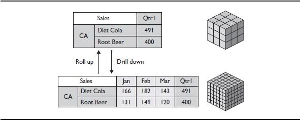
Figure 8. Drilling down and rolling up values in a cube
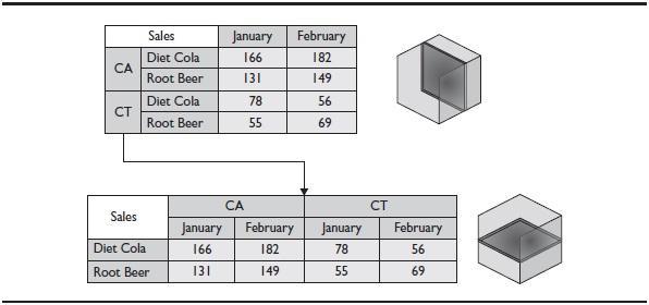
Figure 9. Rotating the cube
Pivot
Pivoting lets you change the orientation of a report. For example, you can move a dimension from a row to a column. Conceptually, pivoting can be thought of as rotating the cube to view analytic data from different perspectives. Figure 9 shows how you can change the visualization of sales data by pivoting the Markets dimension.
You can also use pivoting to move a dimension off the grid to the page. When a dimension is on the page, it acts as a report filter, filtering data visible on the current page by the selected member.
Slicing and Dicing Data
The ability to remove or retain subsets of members on a dimension is a hallmark of an OLAP reporting application. Often, the entire cube is enormous - much larger than can be effectively presented to the user at one time. The OLAP engine allows you to select a subset of data to be presented to the user, as shown in Figure 10.
Oracle OLAP implements slice and dice functionality using a powerful "selection" capability that allows you to determine which dimension values are to be displayed. Essbase uses the intuitive Keep Only action to focus on in a selected subset and the Remove Only action to remove the subset selected from the current view of data. While these differences are located in the front-end client tools, not
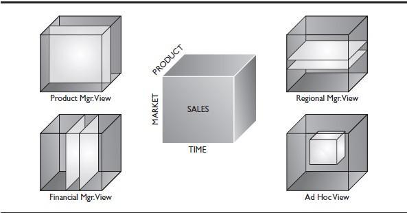
Figure 10. Slices of data in a cube
the engines themselves, differences in the API calls for Oracle OLAP and Essbase influence the capabilities exposed to end users.
Summary of Common OLAP Themes
You should now have a better understanding of OLAP concepts in general and how Oracle OLAP and Essbase implement those concepts. Table 1 summarizes these OLAP concepts and maps them to the terms used by Oracle OLAP and Essbase.
Each product offers full OLAP capabilities; only the implementations are different. Most of the differences in implementation stem from the different approaches taken by the products. The difference in approach is best understood within the context of the origins and evolution of the products. The next two sections summarize the history of Oracle OLAP and Essbase.
| OLAP Concept | Oracle OLAP Terms | Essbase Terms |
| Cube | Cubes, cube-organized materialized views | Multidimensional database, cube |
| Dimension | Dimension | Dimension |
| Dimension member | Dimension member | Dimension member shared member |
| Dimension hierarchy | Hierarchy, current hierarchy,level-based hierarchy, valuebased hierarchy | Hierarchy, alternate hierarchy |
| Hierarchy level | Levels (user-defined), valuebased hierarchy | Levels (automatic or user-defined), generations |
| Member relationships within a hierarchy | Ancestor, parent, sibling, child, descendant | Ancestor, parent, sibling,child, descendant |
| Attribute | Attribute | User-defined attribute (UDA), Attribute dimension |
| Alternate hierarchy | Hierarchy, current hierarchy,level-based hierarchy, valuebased hierarchy | Alternate hierarchy,attribute dimension, hierarchy of shared members |
| Measure | Measure, stored measure | Data value, stored value, Accounts dimension type |
| Calculated measure | Calculated measure | Calculated value |
| Aggregation | Aggregation, aggregation operators | Consolidation, consolidation operators |
| Density and sparsity | Dense, sparse, compressed composites | Dense, sparse, block storage, aggregate storage |
| Drill | Drill up, drill down | Zoom out/drill up, zoom in/drill down |
| Pivot | Pivot | Pivot, point of view |
| Slice and dice | Selection capability | Keep Only and Remove Only |
TABLE 1. Mapping OLAP Concepts to Oracle OLAP and Essbase
The History of Oracle OLAP
Oracle OLAP has a rich history extending back before the advent of relational databases. It grew out of a business need to represent business data in a form that could be easily analyzed. It has gone through several changes over the decades.
This section reviews the history of Oracle OLAP, from its Express days to its current status as the multidimensional component of Oracle's flagship database, the Oracle OLAP option to Oracle Database Enterprise Edition.
Why a Multidimensional Database?
In the late 1960s, Jay Wurts, a student at Massachusetts Institute of Technology (MIT) was working on a project for his professor, John Little. When calculating how much should be spent on advertising for cookies, Wurts found that he spent most of his time wrestling with reformatting the data for his analysis, not on the statistical algorithms or the true data analysis. He realized that he needed some sort of computer-based analytical tool bench for supporting decision making. If the data model could be abstracted from the data itself, the system could be used for a wide array of projects, instead of starting from scratch each time.
Wurts found that once he had modeled the data in a multidimensional form, he was able to report the data in many different formats. By abstracting the data model from the data itself, his system could produce reports that were not part of the original specifications. The user could work with the data in an ad hoc fashion, asking questions that had not been formulated when developing the specifications, on data that was not even loaded when the system was first constructed. Wurts's system allowed users to interact with the data using meaningful names, such as regions, products, months, and so on. Enhancing the system to store numbers with more precision allowed the same engine to be used for financial analysis as well, opening up the software product to a new set of customers.
1960s to 1985 - Glory Days of Mainframe Express
In the early 1970s, Wurts and others in the MIT community - including John Little, Glen Urban, and Len Lodish - formed the company Management Decision Systems (MDS) in Weston, Massachusetts, outside of Boston. They developed Wurts's original multidimensional engine into the product called Express. In the Express environment, arrays can be manipulated with a fourth-generation language (4GL) to conduct business analysis and build systems that help support business decisions, a class of applications then called decision support systems (DSSs). Eventually, this product would be called Mainframe Express.
Mainframe Express was delivered on the IBM VM/CMS, and then Primos platforms in the 1970s and 1 980s. Over the years, advanced capabilities were added to Mainframe Express as it developed into a full-fledged decision-support calculation engine. These included advanced linear-programming capabilities, Box-Jenkins modeling, goal-seeking and a LIMIT command to scope down further commands in a session to subsets of the storage array, and embedded total dimensions for handling multiple levels of a hierarchy in a single structure. Built in this environment were applications such as EasyTrac, a general-purpose DSS application, and Easycast, a general-purpose forecasting product.
1985 to 1990 - A New C-Based Engine
By the mid-1980s, it was time for Express to move to a more modern development environment. Originally written in the AED programming language, Express was rewritten in the C programming language, which was popular at that time. This allowed MDS to attract talented programmers to work on Express. It also allowed MDS to port Express to additional operating systems and hardware platforms, including the increasingly popular IBM PC.
At the same time, MDS recognized that it needed a more sophisticated method of storing data to deal with issues such as inserting new dimension values without needing to rewrite the entire array (a process called shuffling). This new engine was first delivered in 1986 on the MS-DOS operating system as pcEXPRESS version 1.0. As demand for larger databases grew, the limitations of the PC hardware became apparent. This new C-based engine was ported to several operating systems and servers, including VM/CMS, MVS/TSO, VMS, and several variations of UNIX. The product was called pcEXPRESS on the PC platform and Express MDB on other platforms.
Express became dominant in consumer packaged goods companies due to its flexible query capabilities and speed. Many of these companies were also customers of Information Resources, Inc. (IRI), a Chicago-based syndicated data company. IRI had been delivering its supermarket sales data in volumes of books called the Marketing Fact Book. By the mid-1980s, it was looking for a way to deliver its sales data in a new interactive manner. IRI wanted its users to be able to drill down on reports and make the experience of using the data more interactive. IRI purchased MDS in 1985, leaving the Express development staff in the Boston area.
Applications written in Express, especially those targeted to consumer packaged goods companies, became very important to IRI. Express was the underlying technology for EasyTrac, later named DataServer by IRI. In the first releases of EasyTrac/DataServer, pcEXPRESS was used as the front end, providing the ability to navigate through dimensions in a rich environment, and using Mainframe Express and then Express MDB to manage the data using a client/server model. DataServer would become the major delivery vehicle for IRI's new InfoScan data service, which replaced the Marketing Fact Book. Other applications were developed as well, most notably Financial Management System (FMS), a distributed budgeting and planning application.
Between versions 1.0 and 5.0, the pcEXPRESS/Express MDB engine eventually gained the same sophisticated capabilities as Mainframe Express, including selfordering models that would intelligently figure out the order in which equations needed to be solved to calculate a model, and seasonally adjusted forecasting algorithms, such as Holt-Winters.
1990 to 1996 - Express Goes GUI
pcEXPRESS was designed with a character-based user interface - 80 characters by 25 lines. Data was presented in scrollable tables, and the keyboard was used for navigation. The end user could enter graphics mode to display graphs, but true interaction with graphs was limited. Express MDB had only a command-line interface. As personal computer hardware evolved to support graphical user interfaces (GUIs), users began demanding GUIs and the ability to use a mouse with applications. An Executive Information System (EIS) product was offered as a general-purpose tool for finance departments that operated entirely in graphics mode.
To address demands for a richer client interface, IRI started building applications with entirely separate GUIs using Visual Basic and C. Applications were rewritten in this object-oriented GUI environment. The two most successful applications included Financial Management System and SalesAnalyzer (successor to DataServer). Additional applications with analysis capabilities were developed using IRI's data, including SalesPartner, an expert system for fact-based selling; Coverstory, a tool for automatically producing board-room-ready presentations; and BrandPartner for fact-based marketing.
During these years, Express competed head-to-head with Essbase. Essbase touted its intuitive spreadsheet interface. Express touted its strong multicube storage model.
1995 to 1997 - Oracle Buys and Markets Express
In 1995, IRI was looking for cash to retire debt and fund its international expansion. At the same time, Oracle Corporation wanted to augment the data warehouse capabilities in its relational database with OLAP technology. OLAP applications require a multidimensional view of the data, star schemas, and interrow joins for time comparisons and share calculations. Express seemed to fit the bill perfectly. Oracle ended up buying the Express product line and related applications, leaving IRI's syndicated data service with IRI. In effect, Oracle bought IRI's Boston-based products, applications, and development organization. DataServer and SalesAnalyzer were renamed to Oracle Sales Analyzer and sold as a very effective general-purpose performance analysis application. Financial Management System was renamed to Oracle Financial Analyzer (OFA) and sold as a very effective financial analysis and distributed budgeting application.
From 1995 to 1997, Oracle ran the Express products group as a separate group. In this time period, Express Server version 6.0 was delivered as a database service. As a database service, Express Server could deliver data to multiple sessions at once, address more memory, and scale much more than the previous platform would allow. Oracle also continued to enhance the Express platform. Oracle Express Objects (OEO) and its companion, Oracle Express Analyzer (OEA), were designed to allow developers to build applications using popular object-oriented techniques.
A new language, Express Basic (modeled after Microsoft's Visual Basic), was the host language for OEO and OEA, controlling events and the graphical presentation of data. Even the development of Express databases went graphical with the release of Express Administrator, the first graphical tool for developing Express databases.
Around this time, the World Wide Web became a dominant theme in user interfaces. A new API for building web-based applications called Express Web Agent was developed. This API was modeled after Oracle Web Agent and used an HTML template approach combined with Java applets to deliver very functional applications for running on a web server. The Java applets added higher-level objects like pivot table and charts. Programming in this environment leveraged the Express 4GL, the same language used to develop other Express-based applications.
1998 to 2001 - Integrating Express into the Oracle Database
Oracle customers wanted their multidimensional data housed in the Oracle Database, not in the stand-alone Express Server. Oracle decided to start an ambitious project - the true integration of the Express engine directly into the Oracle Database. The C-based Express environment was absorbed into the Oracle kernel and was marketed as the Oracle OLAP option to the Oracle Database Enterprise Edition. This technically challenging project took several years and several releases to develop. The result is a true multidimensional engine embedded and integrated into the heart of the Oracle Database.
2002 to 2003 - Oracle9/OLAP
In the first release of Oracle9i OLAP, OLAP data was still stored in a separate file with a .db extension. At first, Oracle OLAP could be used in ROLAP mode, with data stored in relational tables, or in MOLAP mode, with data stored in true arrays. Use of Oracle OLAP in ROLAP mode was met with limited success, with slow response times for cubes of any significant size.
In Oracle9i Database Release 2, Oracle capitalized on its new object technology in the database to store multidimensional data in a new analytic workspace - a binary large object (BLOB) inside an Oracle table. This allowed OLAP data to be managed, secured, and backed up just like other data in an Oracle database. The BLOB abstraction allowed the data to continue to be stored in arrays and to retain the true multidimensional characteristics from Express.
The application AWM allowed cube designers to create and maintain cubes. AWM provided a graphical environment for defining dimensions and variables, and for mapping to relational tables to source data. Since Oracle tables were the most likely source of data, AWM included a graphical interface for mapping source relational tables to multidimensional objects.
A new API, the Java OLAP API, was developed to give an interface to the multidimensional data. With the declining popularity of object-oriented programming environments, Oracle moved away from its OEO platform and focused its efforts on a new Java-oriented development environment, Business Intelligence Beans (BI Beans), which served as a more approachable programming interface to the Java OLAP API. BI Beans was delivered with Oracle's integrated development environment (IDE) for Java, JDeveloper. Oracle had no generic ad hoc reporting solution at the time, preferring to promote the development of custom applications using BI Beans and JDeveloper. Alternatively, customers could develop web-based applications using Oracle OLAP Web Agent, a web-based programming environment that was a simple port from Express Web Agent, but this environment was not widely promoted or deployed.
2004 to 2006 - Oracle OLAP 10g
With the Oracle Database 10g release of OLAP, Oracle added more capabilities to the language and started the true integration work to bring the multidimensional metadata into the Oracle Database. Compression and dynamic models were added to the aggregation engine. A series of relational tables, the OLAP Catalog, allowed multidimensional objects to be exposed to relational applications. In Oracle Database 10g Release 2, Oracle truly had a platform on which relational applications could issue SQL against multidimensional objects. Again, Oracle turned to its object technology to expose multidimensional objects as a series of rows in a table, using the new function OLAP_TABLE. Oracle also released a plug-in for AWM that built views for accessing Oracle OLAP data using the OLAP_TABLE function. OLAP_TABLE enabled Oracle to establish SQL as the dominant method for accessing Oracle OLAP cubes.
While some companies developed their own custom applications using BI Beans, it became clear that Oracle needed its own ad hoc tool for accessing Oracle OLAP data. Oracle had a sample application that it delivered with BI Beans that some consulting companies developed into an ad hoc reporting tool, including Vlamis Software Solutions VSS Business Analyzer. Oracle used BI Beans to develop its own ad hoc tool for accessing Oracle OLAP cubes in 2004, extending its Discoverer product to include a sister product, Discoverer Plus OLAP. Web-based Discoverer Viewer was also extended to access Oracle OLAP data. At the time of this writing, Discoverer is now marketed as Oracle Business Intelligence Standard Edition. Using the same BI Beans technology, Oracle also released the BI Spreadsheet Add-in, which enabled access to Oracle OLAP cubes directly from Microsoft Excel.
In 2006, Oracle completed its acquisition of Siebel. Siebel had previously purchased nQuire and was using its ad hoc and dashboard tools to provide analytics in its popular CRM applications. Oracle quickly embraced the nQuire tools, branding them as Oracle Business Intelligence Enterprise Edition (OBIEE). At the time of this writing, OBIEE is Oracle's strategic platform for BI applications. Oracle OLAP (and Essbase) data can be reported and analyzed using OBIEE. OBIEE 11g will include additional OLAP reporting and analysis capabilities.
2007 to 2009 - Oracle OLAP 11 g
With the release of Oracle Database 11 g, Oracle took another major step in integrating multidimensional data into the relational engine and support for SQL access to Oracle OLAP cubes. Oracle's customers increasingly need the ability to store summary data from a data warehouse into summary tables.
In Oracle Database 11 g, Oracle extended its materialized view logic to treat OLAP cubes as materialized views. The Oracle optimizer now knows about a "cube scan" operation that can greatly speed up SQL queries against fact tables by rewriting queries to run against cubes with summary data. Oracle created a new function, CUBE_VIEW, which directly reads the OLAP metadata to expose multidimensional data as relational views. Oracle OLAP 11 g also automatically creates views to expose dimensions and cubes as relational views with a star schema. SQL-based applications can now access Oracle OLAP data and calculations as easily as selecting from a series of tables. In addition, dimensions, cubes, levels, hierarchies, and other OLAP metadata are now integrated into the Oracle dictionary. With this version, Oracle OLAP is truly integrated into the Oracle Database.
2009 and Beyond
Oracle OLAP is clearly influenced by its history. Over the years, the original Express 4GL language has been augmented considerably, yet still retains full application development and advanced calculation capabilities as the OLAP DML. The Oracle Database is now positioned as a rich analytic engine, with multidimensional data types, and SQL access to all of these calculations for analytical applications. In addition, a third party, Simba Technologies, has opened up access to Oracle OLAP cubes using the Multidimensional Expressions (MDX) query language from MDX- based tools such as Microsoft Excel. Oracle OLAP can be used as a calculation engine, or especially with cube-organized materialized views, as a sophisticated aggregation engine for a data warehouse.
The History of Essbase
Essbase was released in 1 992 by Arbor Software. Like most successful products, Essbase was invented to address an urgent business need. It has endured and flourished because it fulfilled the need in the right way. We start our discussion of the history of Essbase by reviewing the original problems. Then we show how Essbase solved these problems using a multidimensional approach. Finally, we wrap up our discussion with a summary of important dates in Essbase history, ending with the acquisition of Hyperion Solutions (and Essbase) by Oracle.
Why Essbase?
Essbase was developed as a solution to the two main issues with electronic spreadsheets, called spreadsheet hell and spread marts by those who have experienced them. Both issues arise from the limitations of spreadsheets.
Spreadsheet Hell
Spreadsheet hell comes about as a side effect of the nature of spreadsheets themselves. Spreadsheets excel at capturing two dimensions. After all, spreadsheets are essentially a group of rows and columns. Figure 11 shows how two dimensions, Time and Measures, can be used to model a few data values in a spreadsheet.
In Figure 11, the row and column dimensions (Measures and Time) are used to track income and expense by month and quarter. The challenge is that organizations never model by just two dimensions. What if the company that owned this spreadsheet wanted to understand these values by market as well? The concept of a workbook containing multiple spreadsheets enabled analysts to include a third dimension by adding a new spreadsheet for each member in the dimension. Figure 12 shows how the company ends up with four additional spreadsheets (one for each region) when the Market dimension is included.
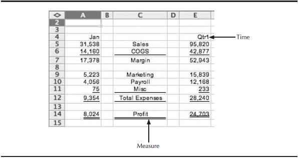
Figure 11. Two dimensions: Measures by Time

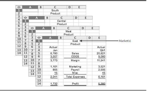
FIGURE 12. Three dimensions: Measures by Time by Market
You may be thinking that five spreadsheets (the original one plus the four regional spreadsheets) are not exactly a burden. But what if the company were to add products to the picture? Figure 13 shows what happens when the company adds five product groupings by the four geographic regions.

Figure 13. Four dimensions: Measures by Time by Market by Product

| Dimension | Input Values | Aggregate Values | Total Number of Cells | Spreadsheet Representation |
| Time | 12 | 5 | 17 | Column |
| Measures | 9 | 9 | 18 | Row |
| Markets | 20 | 5 | 25 | Page |
| Products | 14 | 5 | 19 | Page |
| Scenarios | 2 | 2 | 4 | Page |
Table 2. Five Dimensions Represented in Spreadsheets
In fact, most subject areas are analyzed by several dimensions, and this is where spreadsheets will typically bog down. As we move beyond four dimensions, it becomes increasingly difficult to represent the spreadsheets as images. To show five dimensions, we can use a table format. Table 2 represents five dimensions: the previous four plus a new one called Scenarios.
The Input Values column in Table 2 contains the number of cells that have a data value input for each dimension. For example, in the Time dimension, we have 12 months, hence the value 12 in the table. In the Aggregate Values column, we show how many aggregate values are associated with the dimension. Recall that a typical Time dimension represents a year with four quarters, where the value for each quarter is the sum of the months within the quarter, and the value for the year is the sum of the four quarters. Therefore, the dimension has five aggregate values (4 + 1). The total number of cells is the number of input values plus the number of aggregate values. In the last column, we identify where the dimension was represented in our original spreadsheet example. Recall that Time and Measures were the original column and row dimensions. Markets, Products, and Scenarios are what we call page dimensions. Each page dimension requires that a new spreadsheet be created for every member in the dimension.
On the surface, this example appears fairly simple. But let's do a bit of arithmetic. Beginning with the row and column dimensions, we multiply the number of members for Time and Measures (17 * 18) to arrive at 306 cells in a page. For the page dimensions, we multiply the members belonging to Markets, Products, and Scenarios (25 * 19 * 4) for a total of 1,900 spreadsheets. The result is 581,400 (306 * 1,900) data cells spread over 1,900 spreadsheets!
Spread Marts
Maintaining vital information across spreadsheets is often a tremendous challenge for organizations, large or small. For instance, if the definition of Total Expenses in the previous section's example were modified, the analyst would need to change each of the two calculations under January and Quarter 1 across all 1,900 spreadsheets. That is quite a lot of work and presents many potential sources for error.
Many IT people call data maintained in this fashion "spread marts," because the collection of spreadsheets often becomes a bit of a data mart, housing quite a lot of very important information. Unfortunately, that is where the "mart" comparison ends. A data mart is a collection of data available to many users, stored in a highly scalable database, along a specific subject area. In contrast, spreadsheets are personal productivity tools that allow users to model smaller amounts of data.
Essbase: A Multidimensional Solution
The inventors of Essbase decided to solve the dual problems of spreadsheet hell and spread marts by implementing a database and storing data in terms of dimensions.
In fact, Essbase is an acronym for Extended Spread Sheet dataBase. Their idea was to create a database from a series of disconnected and often single-user-based files and use a spreadsheet tool like Lotus 1-2-3 or Microsoft Excel for query and report creation.
According to United States Patent 5,359,724, Essbase is defined as a "method and apparatus for storing and retrieving multi-dimensional data in computer memory." Essentially, this means that Essbase is a multidimensional database management system (MDBMS). Unlike a relational database management system (RDBMS), Essbase stores data much like a spreadsheet. However, where spreadsheets store values per the combination of just two dimensions (row and column), Essbase allows users to define the number of dimensions that are appropriate for the business case.
Returning to our example, Figure 1, shows the same dimensions - Measures by Products, Time, and Markets - represented as a cube. Each of the dimension members are combined to create a potential data cell that can contains a value. In other words, the combination of specific Product, Market, and Time members yields a value; for example, 267 units of fruit soda sold in California in January.
The great thing about an MDBMS is that you can select the dimensions you want, and the data cells and their relationships are created automatically. For example, you could query the database to create a report containing values for measures by time for a particular market and product, and using a specific scenario. Recall that, for our simple example, we calculated that you would need to create and save 1,900 spreadsheets to model these same five dimensions. Essbase allows you to create any of those 1,900 spreadsheets instantly, simply by querying the multidimensional database for the members you want to display in a spreadsheet.
1992 to 1994 - Essbase Is Born
Essbase was patented on March 30, 1992. Though revolutionary at the time, initial releases of Essbase allowed for fairly small data sets to be stored in Essbase cubes. The cubes were stored on a server, and initially Lotus 1-2-3 and Microsoft Excel
were the primary client-side query and reporting methods. A very rudimentary, script-based report writer was also included.
When first released, the Essbase Server was available only on OS/2. Windows and UNIX support followed shortly thereafter.
Application development and administration were achieved via a Windows- based studio called Essbase Application Manager. With the Application Manager's easy-to-use, drag-and-drop style interface, the power user could create applications without the help of IT. This represented an important major shift in application development.
1994 to 1998 - APIs and the Essbase Web Gateway
The second half of the decade brought a host of improvements and innovation to Essbase. Arbor Software developers saw themselves as engineers of the best MDBMS available. Therefore, instead of creating proprietary reporting tools, the norm for RDBMS at the time, they created and nurtured a partner ecosystem. The approach was to open Essbase to other software developers. The mission was to ensure that Essbase could be integrated into just about anything that needed an MDBMS.
To achieve this mission, Arbor published a series of APIs, enabling both customers and partners to create complementary applications. Next, Arbor Software released the Essbase Web Gateway, a development environment that enabled developers to deliver browser-based applications on top of Essbase.
The Essbase Web Gateway was used to develop and deploy intranet- and Internet- based web-enabled applications for ad hoc analysis, management reporting, enterprise information systems, budgeting, and sales forecasting. Essbase and the Essbase Web Gateway enabled corporations to deliver OLAP applications directly from operational systems or within an overall data warehousing architecture.
1998 to 2003 - New Reporting Options for essbase
After Arbor Software merged with Hyperion Solutions in 1998, several new Hyperion-based reporting options appeared. Hyperion's approach to the software market was very different from Arbor's. After all, Hyperion was an applications vendor, rather than a software engineering company. This would cause some growing pains. The marriage eventually bore fruit, however, as Essbase was used to power some Hyperion applications, as well as to provide extensibility for many of Hyperion's other applications.
By 2002, Hyperion Solutions had evolved a business strategy to help companies better understand their performance. Hyperion, through thought leadership, created the term business performance management (BPM). Gartner later recognized BPM as a category of software called corporate performance management (CPM). Today we might know this better as enterprise performance management (EPM).
2003 to 2007 - Aggregate Storage and Hybrid Architecture
When it first came out, Essbase had one storage type: block storage (BSO). BSO was relegated to a subset of multidimensional applications, due to size constraints. As such, Essbase was well positioned to assist in applications of a more financial nature. Additionally, spreadsheet problems were typically found in the finance department of an organization. This makes sense, as finance users use spreadsheets extensively.
During late 2003 and early 2004, developers undertook a project to create a new form of Essbase storage specifically designed to address applications requiring extensive dimensionality and small update windows. By increasing the amount of data and expanding the number of dimensions and members, Essbase could address a far wider range of applications. This new form of storage was eventually named aggregate storage (ASO). With ASO, most of the data limitations associated with BSO were addressed, so customers could create applications far outside the traditional realm of finance.
A third form of storage, called advanced relational access (ARA), was added with Essbase 9. ARA enabled a hybrid approach to OLAP using Essbase. Whereas BSO and ASO store all the data in their respective Essbase databases, ARA provides for the ability to link back to a relational database. Essentially, you can decide which information along a dimension was stored in the Essbase database versus what was left behind in the relational database. For example, you might drill down through a Time dimension from years to quarters to months. Then, when drilling down from months to days, Essbase queries the relational database and presents the data as though it had been in Essbase the whole time.
Actually, the aforementioned Essbase 9 had been renamed just as Essbase won an award. The new name was Hyperion System 9 BI+ Analytic Services. Over time, it became apparent that the user community preferred and continued to use the former name Essbase. And the recognition that Essbase achieved? Information Age magazine named Essbase as one of "The 10 Most Influential Innovations."
2007 to Present - Essbase Powers Oracle EPM and BI
July 2007 brought the legal entity merge of Hyperion Solutions into Oracle. Many companies "run" themselves via enterprise resource planning (ERP) systems such as Oracle or SAP. However, many of these same organizations used the Hyperion performance management applications to gather information from the ERP systems to provide information to management. So, it was logical for Oracle to join forces with such a complementary vendor. With Hyperion integrated into Oracle, a complete set of offerings would be available. In addition, Hyperion's BPM strategy was recognized by Gartner and, in turn, by Oracle.
Since the acquisition, Oracle has restored the Essbase brand and released Essbase versions 9.3.1 and 11.1.1. Essbase was core to the Hyperion acquisition by Oracle and has since become Oracle's strategic direction for EPM, powering Oracle Enterprise Performance Management System and functioning as a data source for OBIEE Plus. Although this arrangement was conceived of before the Hyperion acquisition, Oracle developers - backed by a host of Hyperion resources - made tremendous improvements to the integration. At present, Oracle is the leading source of performance management systems, per Gartner.
Conclusion
Oracle OLAP and Essbase both offer robust implementations of OLAP concepts. While the products diverge significantly in how they implement some concepts - for example, in their approaches to cubes, levels, and alternate hierarchies - they are remarkably similar in many other ways, including how they approach the concepts of dimensions, hierarchies, members, user-defined attributes, measures, and aggregation. The histories of each product shed some light on why the approaches to OLAP differ. Essbase grew out of the needs of the line of business, and so all relevant dimensions are available for analysis and calculation in an Essbase database. Oracle OLAP evolved from its origins as a mainframe application into an integrated OLAP solution for the Oracle Database. An Oracle OLAP cube serves to replace a set of single-level materialized views and to provide additional calculations.
An understanding of the history of the products also offers insight into how each fits into Oracle's BI and EPM architectures and possible future roadmaps. Oracle OLAP 11g represents the cumulation of years of work to integrate the Express engine fully into the Oracle Database, providing a truly unique partnership of data warehouse and OLAP capabilities. Oracle OLAP is focused on providing data to SQL-based front-end tools and dimensional tools using MDX such as Microsoft Excel as a natural extension to the Oracle Database. Essbase continues to provide a flexible, stand-alone OLAP server, as well as becoming the OLAP engine that powers the Oracle Enterprise Performance Management System suite of products. Both products can supply OLAP data to the front-end tools available with OBIEE Plus.
In the next article, we turn our attention to the general principles that guide the design of an OLAP solution, as well as product-specific design methodologies. We also present the architectures and components for Essbase and Oracle OLAP.
References
"Oracle Announces Next Generation of Open OLAP Technology." Oracle news release, January 8, 1996.
"Oracle Unveils the Industry's Most Comprehensive Solutions for Data Warehousing." Oracle news release, June 21, 1995.
Information Resources, Inc. Announces $100 Million Asset Sale and Technology Agreement with Oracle Corporation." IRI press release, June 12, 1995.
"Oracle Buys Enterprise Performance Management Leader Hyperion." Oracle news release, March 1,2007.