 So you’re ready to journey into the wonderful world of R! Designed by and for statisticians and data scientists, R has a short but illustrious history.
In the 1990s, Ross Ihaka and Robert Gentleman developed R at the University of Auckland, New Zealand. The Foundation for Statistical Computing supports R, which is growing more popular by the day.
Getting R
If you don’t already have R on your computer, the first thing to do is to download R and install it.
You’ll find the appropriate software on the website of the Comprehensive R Archive Network (CRAN). In your browser, type this web address if you work in Windows:
cran.r-project.org/bin/windows/base
Type this one if you work on the Mac:
cran.r-project.org/bin/macosx
Click the link to download R. This puts a win.exe file in your Windows computer or a pkg file in your Mac. In either case, follow the usual installation procedures. When installation is complete, Windows users see two R icons on their desktop, one for 32-bit processors and one for 64-bit processors (pick the one that's right for you). Mac users see an R icon in their Application folder.
Both addresses provide helpful links to FAQs. The windows-related one also has the link Installation and Other Instructions.
Getting RStudio
Working with R is a lot easier if you do it through an application called RStudio. Computer honchos refer to RStudio as an IDE (Integrated Development Environment). Think of it as a tool that helps you write, edit, run, and keep track of your R code, and as an environment that connects you to a world of helpful hints about R.
Here’s the web address for this terrific tool downloading:
www.rstudio.com/products/rstudio/download
Click the link for the installer for your computer’s operating system — Windows, Mac, or a flavor of Linux — and again follow the usual installation procedures.
After you finish installing R and RStudio, click on your brand-new RStudio icon to open the window shown in Figure 1.
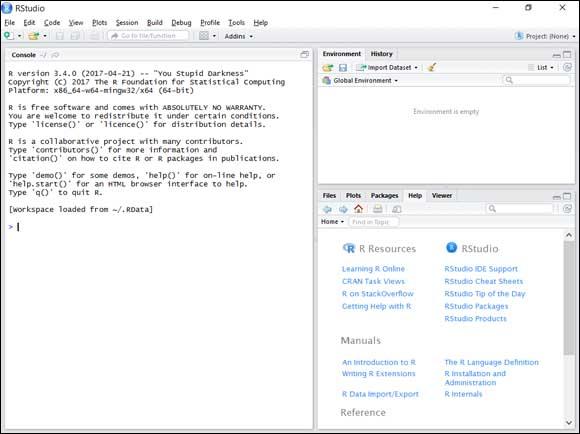
FIGURE 1: RStudio, immediately after you install it and click on its icon.
The large Console pane on the left runs R code. One way to run R code is to type it directly into the Console pane. I show you another in a moment.
The other two panes provide helpful information as you work with R. The Environment/History pane is in the upper right. The Environment tab keeps track of the things you create (which R calls objects) as you work with R. The History tab tracks R code that you enter.
Get used to the word object. Everything in R is an object.The Files/Plots/Packages/Help pane is in the lower right. The Files tab shows files you create. The Plots tab holds graphs you create from your data. The Packages tab shows add-ons (called packages) that have downloaded with R. Bear in mind that downloaded doesn’t mean “ready to use.” To use a package’s capabilities, one more step is necessary, and trust me — you’ll want to use packages.
Figure 2 shows the Packages tab. I discuss packages later in this article.
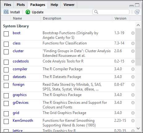
FIGURE 2: The RStudio Packages tab.
The Help tab, shown in Figure 3, links you to a wealth of information about R and RStudio.
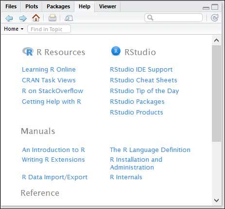
FIGURE 3: The RStudio Help tab.
To tap into the full power of RStudio as an IDE, click the icon in the upper right corner of the Console pane. That changes the appearance of RStudio so that it looks like Figure 4.
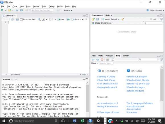
FIGURE 4: RStudio after you click the icon in the upper right corner of the Console pane.
The Console pane relocates to the lower left. The new pane in the upper left is the Scripts pane. You type and edit code in the Scripts pane by pressing Ctrl+R (Command+Enter on the Mac), and then the code executes in the Console pane.
Ctrl+Enter works just like Ctrl+R. You can also highlight lines of code in the Scripts pane and select Code ⇒ Run Selected Line(s) from RStudio’s main menu.
A Session with R
Before you start working, select File ⇒ Save As from the main menu and then save your work file as My First R Session. This relabels the tab in the Scripts pane with the name of the file and adds the .R extension. This also causes the filename (along with the .R extension) to appear on the Files tab.
The working directory
What exactly does R save, and where does R save it? What R saves is called the workspace, which is the environment you're working in. R saves the workspace in the working directory. In Windows, the default working directory is
C:\Users\<User Name>\Documents

On a Mac, it’s

/Users/<User Name>
If you ever forget the path to your working directory, type
> getwd()
in the Console pane, and R returns the path onscreen.
In the Console pane, you don’t type the right-pointing arrowhead at the beginning of the line. That’s a prompt.
My working directory looks like this:
> getwd()

[1] "C:/Users/Joseph Schmuller/Documents
Note the direction the slashes are slanted. They’re opposite to what you typically see in Windows file paths. This is because R uses \ as an escape character — whatever follows the \ means something different from what it usually means. For example, \t in R means Tab key.
You can also write a Windows file path in R as
C:\\Users\\<User Name>\\Documents
If you like, you can change the working directory:
> setwd(<file path>)
Another way to change the working directory is to select Session ⇒ Set Working Directory ⇒ Choose Directory from the main menu.
Getting started
Let's get down to business and start writing R code. In the Scripts pane, type
x <- c(5,10,15,20,25,30,35,40)
and then press Ctrl+R.
That puts this line into the Console pane:
> x <- c(5,10,15,20,25,30,35,40)
As I say in an earlier Tip paragraph, the right-pointing arrowhead (the greater-than sign) is a prompt that R puts in the Console pane. You don’t see it in the Scripts pane.
Here’s what R just did: The arrow-sign says that x gets assigned whatever is to the right of the arrow-sign. Think of the arrow-sign as R’s assignment operator. So the set of numbers 5, 10, 15, 20 … 40 is now assigned to x.
In R-speak, a set of numbers like this is a vector. I tell you more about this concept in the later section “R Structures.”
You can read that line of code as “x gets the vector 5, 10, 15, 20.”
Type x into the Scripts pane and press Ctrl+R, and here’s what you see in the Console pane:
> x

[1] 5 10 15 20 25 30 35 40
The 1 in square brackets is the label for the first line of output. So this signifies that 5 is the first value.
Here you have only one line, of course. What happens when R outputs many values over many lines? Each line gets a bracketed numeric label, and the number corresponds to the first value in the line. For example, if the output consists of 23 values and the eighteenth value is the first one on the second line, the second line begins with [18].
Creating the vector x causes the Environment tab to look like Figure 5.
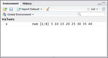
FIGURE 5: The RStudio Environment tab after creating the vector x.
Another way to see the objects in the environment is to type ls() into the Scripts pane and then press Ctrl+R. Or you can type > ls() directly into the Console pane and press Enter. Either way, the result in the Console pane is
[1] "x"
Now you can work with x. First, add all numbers in the vector. Typing sum(x) in the Scripts pane (be sure to follow with Ctrl+R) executes the following line in the Console pane:
> sum(x)

[1] 180
How about the average of the numbers in vector x?
That would involve typing mean(x) in the Scripts pane, which (when followed by Ctrl+R) executes
> mean(x)

[1] 22.5
in the Console pane.
As you type in the Scripts pane or in the Console pane, you see that helpful information pops up. As you become experienced with RStudio, you learn how to use that information.
Variance is a measure of how much a set of numbers differ from their mean. Here's how to use R to calculate variance:
> var(x)

[1] 150
What, exactly, is variance and what does it mean? (Shameless plug alert.) For the answers to these and numerous other questions about statistics and analysis, read one of the most classic works in the English language: Statistical Analysis with R For Dummies (written by yours truly and published by Wiley).
After R executes all these commands, the History tab looks like Figure 6.
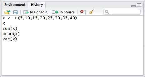
FIGURE 6: The History tab, after creating and working with a vector.
To end a session, select File ⇒ Quit Session from the main menu or press Ctrl+Q. As Figure 7 shows, a dialog box opens and asks what you want to save from the session. Saving the selections enables you to reopen the session where you left off the next time you open RStudio (although the Console pane doesn’t save your work).
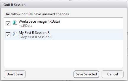
FIGURE 7: The Quit R Session dialog box.
Moving forward, most of the time I don’t say “Type this code into the Scripts pane and press Ctrl+Enter” whenever I take you through an example. I just show you the code and its output, as in the var() example.
Also, sometimes I show code with the > prompt, and sometimes without. Generally, I show the prompt when I want you to see R code and its results. I don’t show the prompt when I just want you to see R code that I create in the Scripts pane.
R Functions
The examples in the preceding section use c(), sum(), and var(). These are three functions built into R. Each one consists of a function name immediately followed by parentheses. Inside the parentheses are arguments. In the context of a function, argument doesn't mean “debate” or “disagreement” or anything like that. It’s the math name for whatever a function operates on.
Sometimes a function takes no arguments (as is the case with ls()). You still include the parentheses.
The functions in the examples I showed you are pretty simple: Supply an argument, and each one gives you a result. Some R functions, however, take more than one argument.
R has a couple of ways for you to deal with multi-argument functions. One way is to list the arguments in the order that they appear in the function’s definition. R calls this positional mapping.
Here’s an example. Remember when I created the vector x?
x <- c(5,10,15,20,25,30,35,40)
Another way to create a vector of those numbers is with the function seq():
> y <- seq(5,40,5)

> y

[1] 5 10 15 20 25 30 35 40
Think of seq() as creating a “sequence.” The first argument to seq() is the number to start the sequence from (5). The second argument is the number that ends the sequence — the number the sequence goes to (40). The third argument is the increment of the sequence — the amount the sequence increases by (5).
If you name the arguments, it doesn't matter how you order them:
> z <- seq(to=40,by=5,from=5)

> z

[1] 5 10 15 20 25 30 35 40
So when you use a function, you can place its arguments out of order, if you name them. R calls this keyword matching. This comes in handy when you use an R function that has many arguments. If you can’t remember their order, use their names, and the function works.
For help on a particular function — seq(), for example — type ?seq. When you run that code, helpful information appears on the Help tab and useful information pops up in a little window right next to where you’re typing.
User-Defined Functions in R
R enables you to create your own functions, and here are the fundamentals on how to do it.
The form of an R function is
myfunction <- function(argument1, argument2, …){

statements

return(object)

}
Here’s a function for dealing with right triangles. Remember them? A right triangle has two sides that form a right angle, and a third side called a hypotenuse. You might also remember that a guy named Pythagoras showed that if one side has length a and the other side has length b, the length of the hypotenuse, c, is
So here’s a simple function called hypotenuse() that takes two numbers a and b, (the lengths of the two sides of a right triangle) and returns c, the length of the hypotenuse:
hypotenuse <- function(a,b){

hyp <- sqrt(a^2+b^2)

return(hyp)

}
Type that code snippet into the Scripts pane and highlight it. Then press Ctrl+Enter. Here's what appears in the Console pane:
> hypotenuse <- function(a,b){

+ hyp <- sqrt(a^2+b^2)

+ return(hyp)

+ }
Each plus sign is a continuation prompt. It just indicates that a line continues from the preceding line.
And here’s how to use the function:
> hypotenuse(3,4)

[1] 5
Writing R functions can encompass way more than I’ve shown you here. To learn more, take a look at R For Dummies, by Andrie de Vries and Joris Meys (Wiley).
Comments in R
A comment is a way of annotating code. Begin a comment with the # symbol, which, as everyone knows, is called an octothorpe. (Wait. What? “Hashtag?” Get atta here!) This symbol tells R to ignore everything to the right of it.
Comments help someone who has to read the code you’ve written. For example:
hypotenuse <- function(a,b){ # list the arguments

hyp <- sqrt(a^2+b^2) # perform the computation

return(hyp) # return the value

}


