Using Oracle Essbase Studio powerful features

The preceding demonstration covered the basic workflow for building, deploying, calculating, and validating an Essbase database. In this blog article, we will address some optional features and more complex functionality available with Oracle Essbase.

We start by introducing two powerful features available with Essbase Studio: drill-through reports and lineage tracking. Then we move from Essbase Studio to Administration Services. We use the Administration Services console to take a closer look at the anatomy of a load rule and show you how to create custom load rules. We then return to the concept of member formulas, introducing the scripting languages and creating a member formula and a calculation script. We wrap up the section with a look at how to use the built-in reporting languages available with Essbase.

Many of the examples in this section use the Sample Basic database, which contains the same data as the TBC1 database used in this article's demonstration.

Creating Drill-Through Reports

Drill-through reports provide one way to implement an HOLAP architecture, where summary data is stored in the Essbase database, but detailed data remains in the relational source. The ability to create a drill-through report is a distinct advantage Essbase Studio has over the traditional load rule approach.

FIGURE 5-9. Smart View finds a drill-through report for Supplier detail.

Understanding How Drill-Through Works

Drill-through is the ability to navigate from your intersection in an Essbase reporting environment to data found in another source. Essbase Studio passes your current context to the other data source. For example, Figure 5-9 shows a typical spreadsheet report for the TBC1 database. When you drill into the cell at the intersection of New York and Root Beer, Oracle Hyperion Smart View checks for the existence of a drill- through report for this data cell and finds one for Supplier detail.

When the report is launched, the context of the data cell—that is, New York and Root Beer—is passed into a SQL statement. The resulting report, shown in Figure 5-10, lists only the suppliers of Root Beer to New York

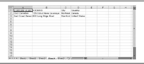
Figure 5-10. The Supplier report lists the suppliers of Root Beer in New York.

Essbase Studio supports the following sources for drill-through reports:

• Relational sources
• URL, standard (manual) or within the template for Oracle Hyperion Financial Data Quality Management (FDM) or for Oracle BI EE
• Custom SQL
• Java method

Creating a Drill-Through Report

To create a drill-through report, follow these steps:

1. In the Metadata Navigator, right-click the Drill Through Reports folder (under SalesAnalysis) and select New | Drill-through Report.
2. Specify a name for the report. For this example, enter Supplier.
3. In the Intersections area, click Add.
4. Expand SalesAnalysis and Hierarchies.
5. Select Product, and then click OK.
6. Change the intersection level to be only Family.

7. Select the Report Contents tab.
8. Add the following columns to the reports (you can drag and drop from either the Data Sources area or the Metadata Navigator): Supplier Alias, Address, City, State, and Zip. 

9. Select the Associations tab.
10. Select SalesAnalysisModel, and then click Save.
11. Select the Report Contents tab.
12. Deselect Show Duplicates in Report, and then click Test.
13.  For Family, enter a value of 200. Press enter and click Show Result. Ensure that the result looks similar to the following report.

      14. Click Close twice.

The report is now available; no further deployment steps are required.

Leveraging Lineage Tracking

The ability to track lineage on an Essbase database and the individual dimensions that make up that database is another advantage of using Essbase Studio. A constant issue with analytical systems is adapting to change. By the time, the data is cleansed and ultimately moved to an analytical database, the needs on the data change. For example, the economic conditions vary, competitive changes alter the business model, or new data sources are identified. In many cases, this results in changes to the analytical structure or the sources upon which it is built. You need to consider what impact a change in structure or source has on your analytical environment. Additionally, after the data models are deployed, you will want to be able to track data from the source to target and back.

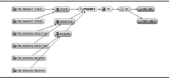
Figure 5-11. Lineage chart for the Market hierarchy

To help solve both of these problems, Essbase Studio provides lineage tracking. Through either the context menu or standard menu selection, you can request lineage diagrams for any metadata element (up to and including deployed models). Figure 5-11 shows a lineage chart for the Market hierarchy. As you can see, the chart displays information back to the original source columns or fields. It also shows the Essbase databases in which the Market dimension is used; in this case, it is used in two Essbase databases TBC and TBC1. Moreover, you also have the ability to review individual object properties from the lineage chart. For example, you can right-click the Market hierarchy object and see specific storage properties.

Creating Custom Load Rules

While Essbase Studio automatically generates rules, you may find yourself in a situation where you want to do a highly custom build or load process on a database. In this case, it may be necessary to use the Data Prep Editor in the Administration Services console to create a load rule directly. Figure 5-12 shows the Administration Services architecture with the Data Prep Editor noted.

A load rule is a mapping object that tells the Essbase server how to read a data source (flat file or relationally based). Load rules have two functions: dimension build and data load. A single rule can perform both functions if required. Let's look at both types, and then create a dimension build rule from scratch.

Dimension Build Rules

The goal of a dimension build rule is to add dimensionality to a database or to alter existing dimensionality. For example, you can use a build rule to update the corporate reporting structure in the database or to add additional SKUs to a product

FIGURE 5-12. Administration Services architecture

dimension. You can have a build rule reorder or incrementally build portions of your database. In addition, a build rule can do something as simple as change an alias on a member.

Figure 5-13 shows a flat file, displayed in Notepad, which we will use as a data source on which to create a dimension build rule. The file, from left to right, presents a hierarchy. In this blog, we introduced the concepts of generations and levels in Essbase. The contents of this file represent generations in a geographic dimension (for example, Market or Regions).

Figure 5-13. Creating a dimension build rule starts with a data source.

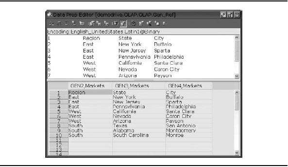
FIGURE 5-14. A dimension build rule maps column headings to members in a hierarchy.

The rule file (shown with a .RUL extension in the database directory) for this data source might look similar to the rule displayed in Figure 5-14.

The Data Prep Editor has two view areas. On the top is the source file in its original state. On the bottom, the load rule shows how Essbase would interpret the data source. For example, the first column should be placed at the second generation of the Markets dimension (GEN2,Markets). The other columns continue to subsequent generations in the hierarchy. In addition, the first line is ignored as a column header and is not built into the model. This is not explicitly shown, but is a simple setting in the rule.

The settings are exactly the same whether you are working with a flat file or querying the metadata directly from a relational source. Essentially, columns in a table are not treated any differently from columns in a file.

Figure 5-15 shows the resulting database outline after this rule is run. Essbase parses the data file and reads it as instructed by the load rule.

This is a very simple example. A dimension build rule can handle much more complex build cases. It can be used to add, ignore, reorder, concatenate, split, or truncate columns. You can also perform string replacements, record selection/rejection,

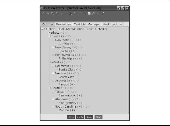
FIGURE 5-15. When run, the database outline is updated to include the hierarchies.

and conversions where required. Furthermore, the rules file does not need to be structured from the top down using generations; you can easily create rules to handle building from the bottom up (levels) through recursive (parent-child) relationships.

Data Rules

You can have load rules that load numeric or textual data into the model. As is the case with dimension build rules, data rules are simply instructions to the Essbase server on how to process the file.

For example, the data source, shown in Figure 5-16, contains columns for each of five dimensions—Market, Product, Scenario, Time, and Measure—plus a Data column. All dimensions are represented for each record (row), and the single numeric fact is listed at the end of each record.

FIGURE 5-16. Flat file with five column headers that map to dimensions

Figure 5-17 shows a sample rules file for this source. The data-load rule simply tells Essbase which dimension to scan in order to find the matching members. For instance, Essbase will look for Jan in the dimension named Year. It is important to note that the last column is specified as the data value. After identifying the specific intersection denoted by the dimension members, Essbase places the value in the Data column into the database at that intersection.

Figure 5-18 illustrates a different data source example. In this case, the Measure members are presented as column headers. The data rule to interpret this data source presentation is shown in Figure 5-19. Notice that this rule handles the Measure dimension differently than in the first example. Each row includes multiple values of the Measures dimension for a single Market-Product-Scenario-Year intersection.

Figure 5-17. Data rule for the preceding data source

Figure 5-18. Flat file with Measures members as column headings

Creating a Load Rule Manually

In this section, we build a load rule that uses a flat file as its data source. The flat file accompanies the Sample Basic database example that ships with Essbase. This is the same sample application used in the Oracle Essbase Database Administrator's Guide. If you do not have this sample, you can download it from the Oracle Technology Network (OTN) web site.

This procedure provides a general guideline for working with load rules. While it focuses on creating a dimension build rule, the process for creating a data rule is similar. For more information, see the Oracle Essbase Database Administrator's Guide.

As was the case with the Essbase Studio example, this procedure is for illustrative purposes only. The specific process to create a custom rule varies based on many factors, including the data source and the type of structure you want to build in the Essbase database.

Finally, it is worth repeating that Essbase Studio eliminates the necessity (in most cases) to create load rules manually, as it generates the load rules based on the actions you take in the Essbase Studio console.

Figure 5-19. Data rule for the second data source

Selecting the Data Source for a Load Rule Follow these steps to start Administration Services and select the data source for the load rule:

1. To start the Administration Services server, select Start | Programs | Oracle EPM System | Essbase | Administration Services | Start Administration Services (Embedded Java Container). If you have the Administration Services server installed as a service in your environment, you can start the service by issuing the specific operating system command or by using the specific operating system user interface. For example, in Windows, open the Services Management console and start the Hyperion Administration Services service.
2. To start the Administration Services console, select Start | Programs | Oracle EPM System | Essbase | Administration Services | Start Administration Services Console.
3. In the Metadata Navigator, expand Essbase Servers, then Applications, then Sample, then Basic.
4. Under demodrive.Sample.Basic, right-click Rules File and select Create Rules File.

       5. The Data Prep Editor appears in the work area of the Administration Services console. Select File | Open Data File. The Open dialog box displays a series of files stored directly on the Essbase Server.

TIP

You can browse to a file located elsewhere by selecting the File System tab of the Open dialog box.

    6. Select Genref.txt and click OK. Genref.txt is a metadata file. There are no numeric data values like those for sales or cost. We will use it to build an outline.

    7. To specify that you are building the outline (not loading data), select View Dimension Build Fields from the toolbar or the View menu.

Specifying File-Based Settings for the Rule Now, you need to specify any file- based settings, such as file headers that you want to skip during the build process. Follow these steps:

1. Select Options | Data Source Properties. The Data Source Properties dialog box appears.

2. The Data Source Properties dialog box lets you specify things like file delimiters and headers, If you need to specify any settings for the data source, do so at this time. For this example, no changes are required. Click Cancel.
3. Select Options | Dimension Build Settings. The Dimension Build Settings dialog box appears.

4. Select the Dimension Build Settings tab. We will add the members in the sample file to the Product dimension.

5. In the Dimension area, double-click Product.

6. In the Build Method area, ensure that Use Generation References is selected and then click OK.

This denotes that this file will build the dimension from the top to the bottom. In this case, the member 500 will be placed toward the top of the outline and subsequent members organized underneath.

Specifying Field Properties for the Rule The next task is to specify field properties, as follows:

1. Select field1 in the Data Prep Editor.
2. Select Field | Properties.
3. In the Field Properties dialog box, select the Dimension Build Properties tab.
4. In the Dimension area, double-click Product.
5. In the Field area, double-click Generation.
6. In the Number area, enter 2. This specifies that the member 500 will be placed directly below the Product dimension name as a product line.

      7. Click Next to move the focus to the next field of the source file.

      8. Repeat the process using the following values for the fields:

     9. When you are finished, click OK.

In the Data Prep Editor, the column headings represent the fields. The headings contain an abbreviation of the Field Type and Field Number (for example, GEN2), followed by the Dimension name (in this case, Product). The values in the table match the values for each of the fields in the original source file.

NOTE If the field labels are not showing, ensure that the Dimension Build Fields option is selected (via the toolbar button or the View menu).

Validating and Saving the Load Rule Follow these steps to validate and save your new load rule:

1. Select Options | Validate. A message tells you whether the rule is valid. Click OK to close the message box.
2. If the rule was not valid, edit the rule and rerun the validation process.
3. To save the load rule, select File | Save. Specify a name for the new load rule.
4. Close the rule.

Executing the Load Rule You can execute the load rule against the database in a couple ways. If you use the Update Outline option (as specified in the following steps), you can test the impact on the database before saving it (this option is available only on block storage databases).

1. Open the Sample Basic outline.
2. Select Outline | Update Outline.
3. Click Find Data File. Browse to and select the original data file, and then click OK.
4. Click Find Rules File. Browse to and select the rule you just created, and then click OK.

5. Click OK. The load rule should complete with a message stating that the file loaded with no errors. Click Close to dismiss this message.

6. Expand the Product dimension in the outline. The additional chain starting with the member 500 should be visible.

  7. If you want to keep the updates, click Save, and then close the outline.

Note that while this rule simply added a chain to an existing dimension, a rule could have been built to create a new dimension in the model.

Load Rules and the SQL Interface

Up to this point, our discussion of custom load rules has concentrated on using flat files for the data source. Quite often, however, load rules are written to source a relational database. The Data Prep Editor provides an interface that lets you connect directly to a relational source. You can create dimensions and load data based on a SQL connection instead of relying on a flat file.

The steps for the creating a rules file from a SQL source are basically the same as those used when creating a standard load rule, after you select the SQL data source. Instead of selecting File | Open Data File, you select File | Open SQL. As shown in Figure 5-20, you then choose the appropriate database source (in this example, the TBC database) from the SQL Data Sources drop-down list.

Figure 5-20. You map a relational source using the Open SQL Data Sources dialog box.

FIGURE 5-21. The SQL data source and associated rule are displayed in the Data Prep Editor.

The SQL data sources drop-down list is populated either by your System DSN list (on Windows) or through use of an ODBC.ini file (UNIX/Linux). You specify the SQL statements that you want to use in the Select, From, and Where portions of the dialog box, and then click OK/Retrieve. After entering your user authentication information, the SQL statement executes, and a portion of the results are displayed in the Data Prep Editor, as shown in Figure 5-21.

All of the remaining steps are the same as for a load file based on a flat file. When using the SQL-based load rule in automation (discussed in detail later in this blog), Essbase executes the SQL embedded in the rule, takes the output from the source, and applies the mappings designated in the rule.

Creating Member Formulas and Calculation Scripts

In our demonstration, the only calculations in the database were the consolidation calculations defined by the hierarchies and an unidentified formula retrieved from the metadata repository. As noted earlier in the article, you can create additional calculations attached to dimension members.

There are two ways to create calculations: through a member formula or through a calculation script. Depending on the nature of what you are doing, you can often accomplish similar tasks with either approach. While there may be slight syntactical differences between commands in member formulas and those in calculation scripts, the general logic and process of creation is similar.

For example, what if 25% of the cost and revenue of Florida is assigned to the East region, while the remainder is assigned to the South. You can easily create a formula with a weighted total to reflect this situation. The formula for the East member might look like this:

@SUM ("New York", "Massachusetts", "Connecticut", "New Hampshire") + ("Florida"*.25);

You would need to create a similar formula for the South member to account for the other 75% of Florida's cost and revenue. In this example, all metrics in the database would be subject to the weighted aggregation. Furthermore, this assignment would apply to all scenarios (Actual, Budget, Forecast, and so forth).

You can expand this formula to include a series of logical tests. The test would validate the intersection and take appropriate actions. For example, you might be considering moving Florida's reporting hierarchy from East to South. You can calculate Actual numbers one way and put a check in to calculate a scenario for reorganization (ReOrg1) in a different way.

IF (@ISMBR("Actual"))

"East"=@SUM ("New York": "New Hampshire");

ElseIf (@ISMBR("ReOrg1"))

"East"=@SUM ("New York", "Massachusetts", "Connecticut",

"New Hampshire") +

("Florida"*.25);

ENDIF

Another common type of calculation (and one used in the following examples) is the creation of variances inside Essbase. For example, if you wanted to create a variance to compare quarter over quarter changes, the formula might look like this:

"Q1 vs Q2"=@VAR("Qtr1","Qtr2");

If you wanted a percentage difference, you could use the @VARPER function instead. (The @VAR and @VARPER functions reverse the variance reporting for items flagged as Expense within the Accounts dimension.)

In the preceding example, the formula would always do a variance between Qtr1 and Qtr2, only. For more flexibility, you could make the formula reusable. For instance, you could build a formula that takes the current quarter and does a variance comparison to the previous quarter.

Calc Scripting Language Versus MDX

This blog described the two database storage methodologies within Essbase: block storage (BSO) and aggregate storage (ASO). Depending on the storage method you choose for a specific database, the language you use to write a member formula is either the native Essbase Calc Scripting Language for block storage databases or the Multidimensional Expressions (MDX) language for aggregate storage databases. The following sections provide a general overview of the language specifications. For detailed information, see the Oracle Essbase Technical Reference.

Block Storage Databases and the Essbase Calc Scripting Language Block storage database formulas use the Calc Scripting Language. This language is a series of functions and commands that lets you select and calculate members of your Essbase database. The Calc Scripting Language is divided into two categories: Commands and Functions.

Commands provide broad capabilities across a database (as opposed to deriving a value for or working with a specific member). For example, you can use the DATACOPY command to copy a slice of data from one portion of the database to another (such as copying last year's actual values to seed this year's budget).

Functions work on individual members, either by selecting a member for calculation or by deriving a value for a member. For example, the @SUM function adds the specified members together. Functions are divided into a series of subcategories. Here is an overview of some of the key areas:

• Boolean These functions are used to perform logical tests on values. For example, they can be used to check if the active member matches a given string, as in @lSMBR("Actual");.
• Relationship These functions retrieve a value from a member in the database based on its relationship to another member. For example, you could request the total sales value for the East market by specifying one of its children, using @PARENTVAL ("New York", "Sales");. This would return the total Sales value for East (the parent of New York).
• Mathematical These functions perform arithmetic and mathematical operations on a member or set of members. For example, you can add a range of values, as in @SUM("Jan":"Mar");.
• Member Set These functions specify a set of members on which to perform actions. For example, to get all of the months in Qtr1 to do an average, you can use @CHILDREN("Qtr1");.

There are also Statistical, Forecasting, Allocations, and a whole host of other categories from which you can choose functions. In total, there are hundreds of prebuilt functions in the Essbase engine.

You should be aware of a few Calc Scripting Language syntax rules:

• Functions must end in a semicolon (;).
• Any member name containing a space, number, or special character (*, &, $, and so forth) must be enclosed in double quotes.
• Functions start with the @ symbol; commands do not.

   

For a complete list of functions, commands, and syntax requirements, see the Oracle Essbase Technical Reference, which is part of the Oracle Essbase documentation set.

Aggregate Storage Databases and MDX When creating formulas for an aggregate storage database, you use MDX. MDX is a standardized query and calculation language for multidimensional databases such as Essbase, Microsoft Analysis Services, and SAP BW. When the aggregate storage option was added to Essbase, MDX was chosen over the Calc Scripting Language in order to embrace the industry-standard query methodology.

Although formulas created in MDX can be used only for aggregate storage databases, MDX can be used to query any Essbase database—block or aggregate storage. This is because the syntax and functions described in this section are universal, regardless of whether they are used in formulas or queries. For more information, see the "Using Essbase Query Languages for Reports" section later in this article.

In general, MDX formulas are very similar to Calc Scripting Language formulas. For example, to perform the same summation we looked at previously, the formula would be SUM([Jan]:[Mar]). Aside from a few apparent syntactical differences, the logic and function are the same.

Unlike the Calc Scripting Language, MDX is not divided into functions and commands. MDX contains a series of functions to perform similar grouping and mathematical operations. MDX functions are organized by action:

• Member return These functions return a member. For example, to see the parent of a Jan, you use the Parentfunction (returns the member Qtr1): [Jan].parent or Parent([Jan]).
• Set return These functions return a set of members. For example, to see the children of Qtr1, you can use the Childrenfunction (returns Jan, Feb, and Mar): [Qtr1].children or Children([Qtr1]).
• Number return These functions are mathematical, such as Average. For example, you can get the average sales for Qtr1 using the Avg function:

Avg([Qtr1].children, [Sales]).

There are many additional functions in the MDX specification. For a complete list of functions, including examples, see the Oracle Essbase Technical Reference in the Oracle Essbase documentation set.

Some syntactical rules for MDX include the following:

• Any member name containing a space, number, or special character (*, &, $, etc) must be enclosed in hard brackets [ ] .
• You can often call a function as a property of a given member by using a dot (.) notation. For example, [Qtr1].children is the same as Children([Qtr1] .

Now let's take a look at how to create a member formula and a calculation script. The following examples are based on the Sample Basic database. Because this database is a block storage database, we use the Calc Scripting Language syntax.

Creating a Member Formula

The sample member formula calculates the variance between Quarter 1 and Quarter 2. Follow these steps to create this member formula:

1. In the Administration Services console, expand Essbase Servers, then your server, then Applications, then Sample, then Basic.
2. Double-click the Outline node to open the Sample Basic outline.
3. Expand the Year dimension.
4. Right-click Qtr4 and select Add Sibling.
5. In the dialog box, type Time Variances. Press the enter key to accept the name, and then press the esc key to leave member-entry mode.
6. Right-click Time Variances and select Add Children.
7. In the dialog box, type Q1 vs Q2. Press the enter key to accept the name, and then press the esc key to leave member-entry mode.

       8. Press and hold the ctrl key and select both Time Variances and Q1 vs Q2.

       9. Click the ~ icon on the toolbar to ensure these do not consolidate on a calculation process.

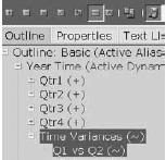
        10. Right-click Q1 vs Q2 and select Edit Properties.

         11. In the Member Properties dialog box, select the Formula tab. The Member Formula Editor is divided into three areas: outline viewer, function selector, and text editor.

         12. In the text editor, type the formula: @VAR("Qtr1", "Qtr2);

     13. Click OK.

     14. In the outline editor, click Save.

     15. If you are prompted to restructure the model, ensure All Data is selected, and then click OK.

Creating a Calculation Script

The sample calculation script clears data on the Budget scenario, copies Actual into Budget, increments the copied values by 5%, focuses the process on the Budget scenario, and then aggregates the new values across the other dimensions. Follow these steps to create this calculation script:

1. In the Administration Services console, right-click the Sample Basic database and select Create | Calculation Script. You will see that the Calculation Script Editor (like the Member Formula Editor) is divided into three areas: outline viewer, function selector, and text editor.
2. In the function selector, select the Alphabetical tab.
3. Expand the tree and double-click FIX. This inserts the FIX command into the script. This command is used to focus the script on a specific subsection of the database.
4. In the text editor, type the remainder of the script to match the following image.

5. On the toolbar, click the Validate button (green checkmark).
6. After validating the script, select File | Save.
7. Name the script, and then click OK.
8. To execute the script, click the Execute button on the toolbar.

Using Essbase Query Languages for Reports

Essbase provides two built-in reporting options: MDX scripts and report scripts. Generally speaking, neither option is normally used in raw format for reporting.

Both MDX and report scripts represent language specifications (similar to SQL) to query data and dimensionality from an Essbase database. Both are often used by front-end reporting tools to interface with an Essbase database. Oracle BI EE, for example, generates MDX queries when sourcing data from Essbase. From a batch processing and automation perspective, you might use either MDX or report scripts to export data from an Essbase database or to validate numbers. This section provides a brief overview of each scripting language.

Querying with MDX

Recall that MDX can be used to query either a block storage or an aggregate storage database. MDX is a standardized query calculation language for OLAP sources. It is similar to the relational database SQL language. An MDX query is divided into three key areas:

• Select This specification denotes what information you want on the axes of your reports. What do you want on rows and columns?
• Data source This specification identifies the Essbase database you are using for the query.
• Where This optional specification filters the results. For example, you could request on data values for April.

Here is a simple MDX query to get all of the Profit subaccount details for the specified market regions in the first quarter:

SELECT Descendants([Profit]) ON ROWS, Children ([Market]) ON COLUMNS FROM
 [Sample.Basic]
WHERE [Qtr1]

FIGURE 5-22. An MDX query and the resulting report

This request can be passed into Smart View via the Execute Free Form MDX Query dialog box. Figure 5-22 shows the formula within this dialog box, followed by the results of the query in Microsoft Excel.

The specific format of the output is determined by the front-end client. MDX does not contain specific formatting functions. Instead, MDX focuses on data and metadata queries.

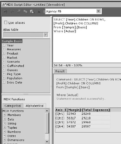
The Administration Services console also includes an MDX editor and viewer. Follow these steps to create a sample MDX query using the Administrative Services console:

1. In the Administration Services console, select File | Editors | MDX Script Editor.
2.  In the text editor, type the following query:

   SELECT [Year].Children ON ROWS,
   
   [Profit].Children ON COLUMNS
   
   FROM [Sample].[Basic]
   
   WHERE [Actual]

   3. From the menu bar, select MDX | Execute Script.

Querying with Report Scripts

Report Script is a legacy Essbase script-based reporting interface. Like MDX, you can use report scripts on either aggregate storage or block storage databases.

The report script language contains functions and is divided into a series of categories:

• Data layout Positioning of a dimension on a report
• Data range Ordering, top, and bottom functions
• Formatting Commands dedicated to specifying overall report formats (such as column width)

The complete report scripts specification is detailed in the Oracle Essbase Technical Reference.

A series of report scripts is included with the Sample Basic database. The following is an example of one of these scripts, which retrieves the top ten products for specified markets:

<Sym

//Suppress shared members from displaying <Supshare

<Column (Scenario, Year)

Actual Budget Jan Dec

<Row (Market, Product)

<Desc Market

//Use bottom level of products

<DimBottom Product

<Top (10, @DataColumn(3))

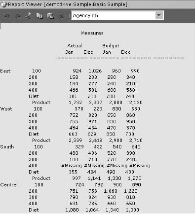
Figure 5-23 shows the output of the script.

Report scripts can be run from the Administration Services console or via the Essbase command-line languages (MaxL and ESSCMD). Regardless of the execution medium, you can send the output of a report script to a file or the screen, or you can stream the results to another program. For example, Financial Reporting (an Oracle reporting tool) issues report script commands to Essbase and displays the data in its user interface.

To create a report script using the Administrative Services console, follow these steps:

This sample report script, when executed, shows the actual and budget values for January and December (as columns) for all market and product combinations (on rows). In the Administration Services console, right-click the Sample Basic database node and select Create | Report Script.

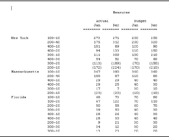
FIGURE 5-23. Report output created by the sample report script

2. In the Report Script text editor, type the following query:

<Sym
<Column (Scenario, Year)
Actual Budget
Jan Dec
<Row (Market, Product)
<Ichild Market
<Ichild Product
!

3. From the menu bar, select File | Save.
4. In the Save dialog box, name the script, and then click Save.
5. Select Options | Execute Script.
6. When prompted, select Console for output, and then click OK.

Вас заинтересует / Intresting for you:

Building Your Essbase Database... 4409 views Ирина Светлова Wed, 02 May 2018, 13:51:28

Understanding Deployment Optio... 1326 views Akmaral Wed, 18 Jul 2018, 07:54:20

Oracle Essbase Care and Mainte... 4708 views Franklin Wed, 22 Aug 2018, 05:48:19

Desirable Functionality in Des... 1413 views Akmaral Sat, 14 Jul 2018, 08:20:48