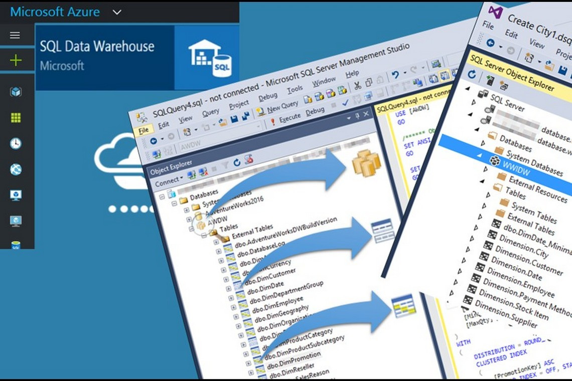

In this blog we will discuss Azure SQL Data Warehouse Table Structures. Note the main features and features. We point out the advantages, as well as possible bottlenecks.
The 5 Concepts of Azure SQL Data Warehouse Tables
- Tables are either Distributed by Hash or Replicated
- The rows of a table are either sorted or unsorted
- Tables are stored physically on disk in either a row or columnarFormat
- Tables can be partitioned
- Tables are either permanent, temporary or external Tables
Above, are some basics about concepts for Azure SQL Data Warehouse tables. The next five pages will cover each point one at a time. This will allow you to see exactly what is going on immediately.
Tables are Either Distributed by Hash or Replicated (1 of 5)
The Azure SQL Data Warehouse gives you two choices for table distribution. These choices are either Hash or Replicated. Large fact tables are usually hashed and smaller tables are usually replicated. When a table is hashed, one of the columns is chosen as the distribution key. In our example above, the Employee_Table (top) is hashed by the Employee_No. The Replicated table (bottom) only has four rows in it and all four rows are on each Node.

Table Rows are Either Sorted or Unsorted (2 of 5)

The rows of a table are either sorted or unsorted. If the table has a clustered index it is sorted, but if it does not have a clustered index then it is unsorted, which is referred to as a heap. You can only have one clustered index per table because you can only sort a table one way. Sorting has nothing to do with a distribution key or a replicated table, but once the rows are placed on a distribution they are then either sorted (clustered index) or unsorted (heap).
Tables are Stored in Either Row or Columnar Format (3 of 5)

A table is stored in either a row format or a columnar format. Traditionally, most systems have always stored the rows of a table in a row format (row store). When a query is run on the table the entire block of rows must be moved from disk into memory, where they are processed. This works well when all columns (or most columns) are needed to satisfy the query. Modern designs of computer systems will often now include a column format (column store). This works extremely well on queries that don’t need all columns (or most columns) to satisfy the query, such as analytics, aggregations, etc. Only the columns needed will then be transferred from disk into memory. The Azure SQL Data Warehouse gives you a choice.
Tables can be Partitioned (4 of 5)

CREATE TABLE Ord_Tbl_Part (

   Order_Number integer
  ,Customer_Number integer
  ,Order_Date  date
  ,Order_Total decimal(10,2))

WITH ( DISTRIBUTION = HASH (Order_Number),

PARTITION ( Order_Date

RANGE RIGHT FOR VALUES

( '2015-01-01','2015-02-01','2015-03-01','2015-04-01',
  '2015-05-01','2015-06-01','2015-07-01','2015-08-01'
 ,'2015-09-01','2015-10-01','2015-11-01','2015-12-01' )));
Above, is the CREATE statement for the Ord_Tbl_Part table. This table is a rowstore table that is partitioned by Order_Date. By using RANGE RIGHT and dates for the boundary values, it puts a month of data in each partition. The distributions each hold different rows, but store each month in their own block(s). This physical partitioning allows for faster loads and faster maintenance (Insert, Update, Deletes). This is the design you want when users are performing range queries on dates.
There are Permanent, Temporary and External Tables (5 of 5)
Permanent Tables – These tables reside permanently and only a DROP or TRUNCATE statement removes them.
Temporary Tables – These tables reside temporarily on the system. Here is more information:
- Global Temp tables are not supported on the Azure SQL Data Warehouse
- When creating
TEMPTable you must specifyLOCATION=USER_DB - Creating
NON CLUSTEREDindexes are not supported on temp tables
External Tables – These tables point to data in a Hadoop cluster or Azure blob storage. External tables are used most often to:
- Query Hadoop data from within the Azure SQL Data Warehouse.
- Import and store Hadoop data into the Azure SQL Data Warehouse by using the
CREATE TABLE AS SELECTstatement.
The Azure SQL Data Warehouse utilizes permanent tables for permanent data, temporary tables for temporary information and external tables in order to query Hadoop and blobs.
Creating a Table With a Distribution Key
CREATE TABLE Emp_Intl (
  Employee_No	INTEGER
  ,Dept_No	SMALLINT
  ,First_Name	 VARCHAR(12)
  ,Last_Name	CHAR(20)
  ,Salary	 DECIMAL(8,2)
) WITH (DISTRIBUTION = HASH (Employee_No)) ; 
Above, is a basic TABLE CREATE STATEMENT for a table with a Distribution Key. You can only use one column as the Distribution Key in the Azure SQL Data Warehouse. The values in this column will be hashed with a hashing formula and used to distribute the rows of the table across the Distributions. Picking a good key is essential. An excellent Distribution Key will allow for even distribution among the many distributions.
Creating a Table that is Replicated
CREATE TABLE Dept_Intl
(
    Dept_No	        INTEGER
   ,Department_Name	VARCHAR(30)
) WITH
(DISTRIBUTION = REPLICATE) ; 
Above, is a basic TABLE CREATE STATEMENT for a table that is replicated across all nodes. That means that the entire table with every row is copied to each and every node. This should be done for relatively small tables because you are in essence duplicating the table on each node. This is done so when a join is performed between this Dept_Intl table and a large Emp_Intl table, the matching rows will be Distribution Local. This means the matching rows are already on the same node and therefore will not have to be shuffled across nodes to make the join happen.
Distributed by Hash vs. Replication

Each node has eight distributions and each distribution has its own set of disks. So, think of this as each node having at least eight disks to place the table rows that it owns. If a table was small, then a node might have all of the rows it owns in a single distribution. This is often the case with a table that is replicated. If a table is huge, then a node might have rows stored in all eight distributions, which is often the case for tables distributed by hash.
The Concept is All About the Joins

The Azure SQL Data Warehouse gives you two choices for table distribution. These choices are either hash or replicated. Large fact tables are usually hashed and smaller tables are usually replicated. The bottom line is that an Azure SQL Data Warehouse needs for two joining rows to be on the same Node. That is why in a 5-table join, an Azure SQL Data Warehouse will join two tables at a time. If tables are replicated, then they are always on the same node as the rows they join. That is why a large Fact table will often be distributed by hash and the smaller tables it joins to will be replicated. The setup of tables on MPP systems are all about the joins.
Creation of a Hash Distributed Table with a Clustered Index

Above, is the CREATE statement for the Claims table. This has a DISTRIBUTION=Hash on Claim_ID. It also has a clustered index on Claim_Date. That means that each node will sort the rows by Claim_Date. This is excellent for range queries. Users will often look up claims based on a time frame, such as per day, week, month, quarter or year.
A Clustered Index Sorts the Data Stored on Disk

A Clustered Index is created to command the Azure SQL Data Warehouse to sort the actual data on disk according to the sorted order of the column values. Each table can have only one clustered index at the same time. For distributed tables, a clustered index affects the way data is stored within each distribution across the nodes, however, it does not affect which rows are assigned to each distribution. For replicated tables, the clustered index affects the way the data is stored within each replicated table, however, it does not affect where the replicated tables are stored. A clustered index sorts the data on disk which is very important for range queries. Above, we created a Clustered Index on Order_Date, so now a full table scan won’t be needed for all queries.
Each Node Has 8 Distributions

Each node has eight distributions and each distribution has its own set of disks. So, think of this as each node having at least eight disks to place the table rows that it owns. Better yet, think of this as each compute node having eight parallel processes (called distributions) with each parallel process having its own dedicated disk.
How Hashed Tables are Stored Among a Single Node

Each node has eight distributions and each distribution has its own set of disks. So, think of this as each node having at least eight disks to place the table rows that it owns. If a table was small, then a node might have all of the rows it owns in a single distribution. If a table is huge, then a node might have rows stored in all eight distributions.
Hashed Tables Will Be Distributed Among All Distributions

Above, we see four nodes and each node has eight distributions for a total of 32 distributions. We also see our five tables. Each table is hashed (in this example) and each table has spread different rows across all 32 distributions. All five tables above are row based tables.
Creation of a Replicated Table
 and each table has spread different rows across all 32 distributions. All five tables above are row based tables. Creation of a Replicated Table")
Above, is the CREATE statement for the Addresses table. This has a DISTRIBUTION=Hash on REPLICATE. This table’s data will be duplicated on each node in its entirety.
How Replicated Tables are Stored Among a Single Node

Each node has eight distributions and each distribution has its own set of disks. So, think of this as each node having at least eight disks to place the table rows that it owns. Replicated tables are duplicated in their entirety across each node. If a table has 20 rows and there are 4 nodes in the system then each node has the same 20 rows. The rows for a replicated table store all the rows only once per node, but the Azure SQL Data Warehouse actually spreads those 20 rows across all eight distributions. This is done using file groups. Above, it appears that the entire table is only on one of the nodes disk, but that is just to illustrate that the entire table is copied only once per node.
Replicated Table will be Duplicated among Each Node

Above, we see four nodes and each node has eight distributions for a total of 32 distributions. We also see four tables. Each table is replicated so each table is thus duplicated across a node one time. All four tables above are row based tables.
Distributed by Replication

With Replication, a table is copied in its entirety to every Azure SQL Data Warehouse compute node. Is this duplicating the table and data across each compute node? Yes! Why in the world would anyone do this? For one reason, The joins! For two rows to be joined they need to be on the same compute node. When the Addresses table joins to the Subscriber table, the replication of the Addresses table will guarantee that the matching rows to the Subscribers will be on the same compute node. Take good advice here and replicate all small table that join to larger tables.
How Hashed and Replicated Tables Work Together

The Fact table (Claims), which is large, will be spread across all eight distributions. The dimension tables (Addresses, Subscribers, Providers and Services) are replicated once on the node. This will allow for easy joining among the five tables.
Tables are Stored as Row-based or Column-based

Above, is a picture of the same table stored as a row-based (top) and column-based design. Notice that either way the node gets the entire row, but the Azure SQL Data Warehouse gives you the option of storing it in either a row-based or column-based design. When a query select all columns in a table the row-based storage if faster, however for queries that only select a few columns the column-based storage if faster. The column-based storage has advanced compression opportunities that save a great deal of space.
Creation of a Columnar Table that is Hashed
CREATE TABLE Sales_Columnar_Hashed
  (
    Product_ID int NOT NULL,
    Sale_Date date,
    Daily_Sales decimal(9,2)
  )
WITH ( DISTRIBUTION = HASH(Product_ID),
CLUSTERED COLUMNSTORE INDEX );
Above, is the CREATE statement for the Sales_Columnar_Hashed table. This table is a columnstore table that is hashed by the Product_ID column. The table has nine rows and three columns. The rows are hashed and the entire row is placed on a distribution, but then it is stored in separate columns. The idea is that when a query is run that can be satisfied by using only one or two of the columns, then the system only has to move that one or two columns from disk to memory.
How Hashed Columnar Tables are Stored on a Single Node

The Addresses table has four columns in it. The Subscribers table has five columns and the Claims table has nine columns. Each column is stored in its own page.
How Hashed Columnar Tables are Stored on All Distributions

Above, we see four nodes and each node has eight distributions for a total of 32 distributions. The Addresses table has four columns in it. The Subscribers table has five columns, and the Claims table has nine columns. All 32 distributions hold a portion of each table, and each table stores each column in a separate page.
Comparing Normal Table Vs. Columnar Tables

Above, is a picture of the same table stored as a row-based (top) and column-based design. Notice that either way the node gets the entire row, but the Azure SQL Data Warehouse has the option of storing it in either a row-based or column-based design.
Columnar can move just One Segment to Memory

Segments on Distributions are Aligned to Rebuild a Row

Why Columnar?

Each data block holds a single column. The row can be rebuilt because everything is aligned perfectly. If someone runs a query that would return the average salary, then only one small data block is moved into memory. The salary block moves into memory where it is processed as fast as lightning. We just cut down on moving large blocks by 80%! Why columnar? Because, like our Yiddish Proverb says, "All data is not kneaded on every query, so that is why it costs so much dough."
Columnar Tables Store Each Column in Separate Pages

This is the same data you saw on the previous page! The difference is that the above is a columnar design. I have color coded this for you. There are 8 rows in the table and five columns. Notice that the entire row stays on the same disk, but each column is a separate block. This is a brilliant design for Ad Hoc queries and analytics because when only a few columns are needed, columnar can move just the columns it needs to. Columnar can't be beat for queries because the pages are so much smaller, and what isn't needed isn't moved.
Visualize the Data – Rows vs. Columns

Both examples above have the same data and the same amount of data. If your applications tend to need to analyze the majority of columns or read the entire table, then a row-based system (top example) can move more data into memory. Columnar tables are advantageous when only a few columns need to be read. This is just one of the reasons that analytics goes with columnar like bread goes with butter. A row-based system must move the entire page into memory even if it only needs to read one row or even a single column. If a user above needed to analyze the Salary, the columnar system would move 80% less block mass.
Creation of a Columnar Table that is Replicated
CREATE TABLE Sales_Columnar_Replicated

  ( Product_ID int NOT NULL,
    Sale_Date date,
    Daily_Sales decimal(9,2))

WITH ( DISTRIBUTION = REPLICATE,

CLUSTERED COLUMNSTORE INDEX );
Above, is the CREATE statement for the Sales_Columnar_Replicated table. This table is a columnstore table that is replicated on each node. The table only has nine rows and three columns. Each table holds the exact same data. It is like looking in a mirror. That is what replicated means. The table is Replicated, but the storage is a columnar (columnstore) design. This allows single columns to be placed into memory for processing.
Creating a Partitioned Table Per Month
CREATE TABLE Ord_Tbl_Part (

  Order_Number integer
 ,Customer_Number integer
 ,Order_Date  date
 ,Order_Total decimal(10,2))

WITH
  (

DISTRIBUTION = HASH (Order_Number),
PARTITION ( Order_Date
RANGE RIGHT FOR VALUES

  (

'2015-01-01','2015-02-01','2015-03-01','2015-04-01',
'2015-05-01','2015-06-01','2015-07-01','2015-08-01'
,'2015-09-01','2015-10-01','2015-11-01','2015-12-01'

)));
Above, is the CREATE statement for the Ord_Tbl_Part table. This table is a rowstore table that is partitioned by Order_Date. By using RANGE RIGHT and dates for the boundary values, it puts a month of data in each partition.
A Visual of One Year of Data with Range Per Month

Above, is a visual of the Ord_Tbl_Part table that was created on the previous page. This table is a rowstore table that is partitioned by Order_Date. By using RANGE RIGHT and dates for the boundary values, it puts a month of data in each partition. This table is NOT replicated, but hashed. The nodes each hold different rows, but store each month in their own block(s). This physical partitioning allows for faster loads and faster maintenance (Insert, Update, Deletes). This is the design you want when users are performing range queries on dates.
Another Create Example of a Partitioned Table
CREATE TABLE Sales_Partitioned

  (
   Product_ID int NOT NULL,
   Sale_Date date,
   Daily_Sales decimal(9,2)
  )

WITH

  (
PARTITION ( Product_ID
RANGE LEFT FOR VALUES (100, 200, 300, 400 )),
CLUSTERED COLUMNSTORE INDEX
  ) ;
Above, is the CREATE statement for the Sales_Partitioned table. This table is a columnstore table that is partitioned by Product_ID. Above, the partitions are listed for both a Left and Right partition of values.
Creating a Partitioned Table Per Month That is a Columnstore
CREATE TABLE Ord_Tbl_Part_Columnar (

   Order_Number integer
  ,Customer_Number integer
  ,Order_Date  date
  ,Order_Total decimal(10,2))

WITH

  (

DISTRIBUTION = HASH (Order_Number),
CLUSTERED COLUMNSTORE INDEX,
PARTITION ( Order_Date
RANGE RIGHT FOR VALUES

  (

'2015-01-01','2015-02-01','2015-03-01','2015-04-01',
'2015-05-01','2015-06-01','2015-07-01','2015-08-01'
,'2015-09-01','2015-10-01','2015-11-01','2015-12-01'

)));
Above, is the CREATE statement for the Ord_Tbl_Part table. This table is a columnstore table that is partitioned by Order_Date. By using RANGE RIGHT and dates for the boundary values, it puts a month of data in each partition.
Visual of Row Partitioning and Columnar Storage

Above, is a visual of the Ord_Tbl_Part_Columnar table that was created on the previous page. This table is a columnar table that is partitioned by Order_Date. This table is NOT replicated, but hashed. The nodes each hold different rows, but store each column and each month in their own block(s). This physical partitioning allows for faster loads and faster maintenance (Insert, Update, Deletes). This is the design you want when users are performing range queries on dates.
CREATE TABLE AS (CTAS) Example
 Example")
Above, is the CREATE statement for the New_Customer_Table_Columnar table, using the column definitions and data from the source table Customer_Table. This new table has been created using the CREATE TABLE AS (CTAS) syntax.
Creating a Temporary Table

SELECT AVG(Salary) as AVGSAL
   FROM #Emp_Temp ;

AVGSAL
------------
46782.153333
You create a local temporary table by using the # prefix before the table name. The temporary table can only be accessed from its own session. You cannot create partitions, views, or non-clustered indexes on a temporary table nor can you have two temporary tables with the same name in the same session.
Facts About Tables
- Tables can be either row oriented (rowstore) or column oriented (columnstore).
- Row-based tables are either distributed by Hash or Replicated. Default is Replicate.
- A row oriented table can have 1 clustered index and up to 999 nonclustered indexes.
- A table created without a clustered columnstore index is stored by row.
- A table with a columnstore index is stored by column.
- A columnstore table has one clustered columnstore index and no other indexes.
- Clustered and nonclustered indexes on any rowstore table can be dropped at any time.
- A columnstore index automatically includes all columns in the table. None of the columns are key columns.
- All Columnstore tables are auto-compressed.
- A clustered columnstore index does not affect how data is distributed across nodes because data is always distributed by rows, but it affects how the data is stored.
Above, are the key facts you need to understand about Azure SQL Data Warehouse tables.