
 Earlier in our blogs, we covered general principles for designing effective OLAP applications. In this article, we expand on those general principles as they apply to the process of designing an Essbase database.
Who Designs Essbase Databases?
As mentioned in this blog, Essbase is often "owned" by line-of-business users, rather than by IT departments. Essbase databases are therefore designed and built either by an Oracle solutions consultant contracted by the line of business or by a business user within the organization itself.
A good candidate for an internal Essbase designer/administrator is someone we call the power business user. You can recognize the power business user in your own organization by the types of activities this employee is currently performing, such as engineering multispreadsheet analyses and creating Microsoft Access applications with macros. Our experience shows that with appropriate training, in-house Essbase designers/administrators are very effective, because they are intimately familiar with the organization's data and needs.
As previously mentioned, designing any OLAP database begins with analyzing existing reports and the data sources that feed those reports. From the reports, you can deduce dimensions and select the dimensions to include in our OLAP model. The Essbase-specific part of the design methodology begins when you create an outline of the model in Essbase. You then validate a label outline with the business users and incorporate feedback. You enhance the label outline with dimension types, data types, and alternate hierarchies. Finally, you decide which type of data storage best suits the model that you have created.
Identifying Data Sources
A common question when first starting to design an Essbase database is "Where do I get my source data and metadata?" A complementary question is "What data sources are supported by Essbase?" Essbase supports the following data sources:
- Flat files (text)
- Spreadsheets (xls)
- Singular relational sources
- Star/snowflake schema
- Extract, transform, and load (ETL) process output (such as from Informatica or Oracle Data Integrator Enterprise Edition)
- API-based data streaming
In short, Essbase is data source-agnostic. If you can provide data output from a system, it can be input into an Essbase database.
Source data and metadata depend on the specific type of analysis the users want to perform and the types of systems in which that information is stored. Many companies have an extensive data warehouse and build Essbase databases directly off the warehouse. Just as many companies store data in a plurality of formats (flat file extracts, data warehouse, departmental relation models, and so on) and build Essbase databases from these federated sources. The source data and metadata for your cpecific Essbase database vary based on the specifics of your deployment environment. From a design perspective, it is important to remember that regardless of its source, data can be consolidated into an Essbase database for reporting and analysis.
Defining the Outline
With the results of the reports analysis in hand, the next step is to create the OLAP model. In Essbase, the design process moves online via one of the console tools: Essbase Studio console, Administration Services console, or Integration Services console. The tool you choose depends on your data source. Essbase Studio can be used for most data sources, while each of the other tools is more specialized.
In the console tool, you map the data sources and model the dimensions and their hierarchies. The outcome of this process is the Essbase outline.
The Essbase outline is, quite simply, a collection of dimensions. It is the fundamental reporting and mathematical structure of your OLAP model. You can view the outlines for all Essbase databases in the Administration Services console. Figure 3-9 shows a sample outline.

Figure 3-9. Sample Essbase outline

Figure 3-10. Sample report based on the dimensions in the preceding outline
Any piece of numeric data provided by this Essbase database is in respect to all dimensions. For example, if you queried the database for sales for the East region in January, the resulting report might look like the spreadsheet in Figure 3-10.
Notice that the dimensions not specified in our query (Product and Scenario) are shown on the point of view (POV). Essbase must represent data in respect to all base dimensions. While we asked for sales in the East for January, we got this result for all products and all scenarios (in this case equivalent to actual). Whenever you get data from, or send data to Essbase, you must represent a member from every dimension.
It is possible that a tool might abstract the display and hide the POV dimensions; nonetheless, if they are not on the grid, they are implied in the result Essbase returns.
The requirement of representing all dimensions is only one way in which the outline dictates the reporting structure. When you refresh an empty spreadsheet in either Oracle Hyperion Smart View for Office or the Oracle Essbase Spreadsheet Add-in, the resulting report is populated with a default retrieval, which is made up of the top of all dimensions and a value, if one exists at that intersection. Figure 3-11 shows a sample report.


Figure 3-11. Default data retrieval shows the top level of all dimensions and a value.

Figure 3-12. Drilling down on a dimension in a report reveals the dimension members.
In this case, the outline dictates dimensional positioning. The first dimension in the outline (Year) is placed in the row, and the second dimension (Measures) is placed on the column. The remaining dimensions are placed on the POV toolbar in the order in which they appear in the outline.
When we drill into the Year dimension, we see the quarters in the year, as shown in Figure 3-12. Figure 3-13 shows the outline that supports the report in Figure 3-12. Notice that the order of the quarters is the same.
We understand the logic inherent in ordering the quarters sequentially. Essbase, however, lets you order them in any manner you desire. If you were to place Qtr1 in between Qtr3 and Qtr4 in the outline, it would affect all reports drilling into that dimension, as shown in Figure 3-14. This affects the default display order only. Essbase still knows that the prior quarter for Qtr 4 is Qtr 3, because Essbase has time intelligence built in. It is important to know that time-series and other calculations would adjust automatically to work with the new structure.
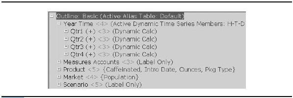
FIGURE 3-13. The outline controls the order in which members are displayed in reports.
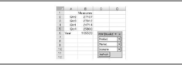
FIGURE 3-14. Changing the order in the outline changes the order in the report.
The outline also controls dimensional math—that is, the aggregation behavior inherent in the hierarchical structure. In Figure 3-13, you can see plus signs (+) to the right of each quarter. These are called consolidation operators or unary operators. In this case, we add the quarters together to derive the value for Year. Essbase also offers built-in time intelligence capabilities.
Design methodology extends beyond the concept of the outline. When building an Essbase database, you must consider data sources and flow, available RAM, user load requirements, and a myriad of other factors. Having said that, the outline is the engine that drives everything in the database. When creating the outline, some thought needs to be given to the order of dimensions (for retrieval), the hierarchy of members (for aggregation), and the order of members at each level (for display purposes).
Validating the Outline with Business Users
The design of the outline is intended to serve the needs of the business user. A common approach to engaging users is to present them with a label-based outline. This lets the designers communicate their understanding of the business requirements and allows the users to see the outline in common terms.
In a label-based outline, you first show the levels that will be defined. You then pick one or two sample values at each level, showing sample drill paths. This helps users relate to the abstract level names, using some well-known values as examples of each level. You can incorporate feedback from this review to improve the outline.
Figure 3-15 shows an example of a label-based outline, with hierarchies for two dimensions: Entity and Products. The first tree under each dimension shows the drill path using general business names. The second tree under each dimension shows a practical example from the data set.

FIGURE 3-15. A sample label-based outline
Enhancing the Outline
Determining the dimensional structures in an outline is key to overall success. However, you also need to consider the following items:
- Di mension types
- Data types
- Alternate views of the data
Remember that design is an iterative process. After enhancing the outline, be sure to validate the changes with business users.
Essbase Dimension Types
By default, dimensions in Essbase have no dimension type (they are tagged as "none"). Untyped dimensions are often called business view dimensions, because they reflect how you view your business. For example, dimensions like Products, Customers, and Regions are common business view dimensions.
Dimension types enhance the analysis you can do across the standard dimensions. Dimension types offer specialized capabilities and have a considerable impact on the design of the model. Essbase calculates time and accounts dimensions before other dimensions.
NOTE
Dimension types in Essbase are optional. It is, however, rare to find an implementation that does not use one or more dimension types.
Accounts Dimension The accounts dimension type is the most widely used. Applying this tag to a dimension lets Essbase know where the majority of the calculations will occur. Only one dimension in an Essbase database can be tagged as an accounts dimension.
NOTE
The use of the term accounts can be a bit misleading. Many people assume that this is a chart of accounts or explicitly financial. This is not the case. Essbase is (at the core) a calculator. While it does contain many functions that are financial in nature, it contains just as many that are statistical or analytical.
The accounts dimension type provides specialized functionality across the members in the selected dimension. Two key capabilities are expense reporting and time balancing.
Expense reporting flips the sign on variance calculations involving expenses. For example, if you have a variance calculation that is Actual-Budget, then you could get a report that looks like this:
| Actual | Budget | Variance | |
| Sales | 100 | 120 | -20 |
| COGS (Expense Reporting) | 100 | 120 | 20 |
Notice that the same calculation derives differently. For Sales, a variance against the budget shows as negative. However, for Cost of Sales (COGS), the variance is in your favor, so it derives as positive. The expense reporting tag handles that logic for you. There is no need to account for it in the logic of the database.
Time balancing specifies how values derive across time. For example, consider Sales and Opening Inventory over time:
| January | February | March | Quarter 1 | |
| Sales | 100 | 120 | 150 | 370 |
| Opening Inventory (Time Balance First) | 50 | 75 | 93 | 50 |
For Sales, the value at Quarter 1 is derived using straightforward aggregation—it is the sum of the months in the quarter. Opening Inventory, on the other hand, requires that the value at Quarter 1 be the same as the value at the beginning of the time period—in this case, the value for January. Essbase provides these time-balance capabilities for the accounts dimension:
- Time Balance First (TB First), which uses the first value in time period
- Time Balance Last (TB Last), which uses the last value in a time period
- Time Balance Average (TB Average), which uses the average values across a time period
- Flow, which lets values flow across years (for example cash on hand)
As the name of the feature implies, time balancing requires a time dimension.
Time Dimension Essbase has a time dimension type for managing time. The specific capabilities of this dimension type vary depending on the nature of your deployment, but in general, time dimensions provide date-differencing and time- aware calculations and selections, as well as period-to-date reporting.
Essbase recognizes that January 21,2008, is a greater overall value compared to January 25, 2007. Essbase provides the ability to count the number of seconds, hours, days, weeks, quarters, months, and years in between those dates. Additionally, Essbase can easily perform parallel period analysis by letting you select comparative time periods. For example, if you want to look at the third day of each week across the year, you can perform simple selections to bring these periods onto a report.
Essbase also lets you provide time-to-date values in reports. For example, you can ask for a sales-to-date summary for May, and Essbase totals the values from January to April as well as May and presents the total (see Figure 3-16). Alternatively, you can ask for sales-to-date values for the quarter, and Essbase adds values for April and May.

Figure 3-16. Sales-to-date summary for the quarter as of May
There are two variations of the time dimension type: the standard time dimension and a date-time dimension. Both types provide the preceding features, but specific capabilities may vary depending on the time dimension variation. For more information, see the Essbase Database Administrators Guide.
Attribute Dimension and Base Dimension Attribute dimensions provide the ability to group members by characteristics. For example, you might have an attribute dimension that groups products by package type or by introduction date. Attribute dimensions are listed at the bottom of a database outline, as shown in Figure 3-17, and identified with the Attribute tag.
Attribute dimensions are assigned to base dimensions. Base dimension simply means any dimension that is not an attribute dimension. In a block storage model, an attribute can be assigned to only a sparse base dimension; in an aggregate storage model, any dimension can be assigned attributes.
In an outline, the attribute dimensions for a given base dimension are listed in braces ({}) next to the base dimension name. For example, in Figure 3-17, the Product dimension has four attribute dimensions assigned to it: Caffeinated, Intro Date, Ounces, and Pkg Type.
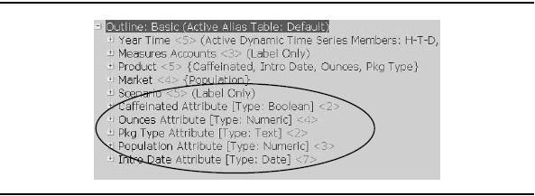
Figure 3-17. Attribute dimensions
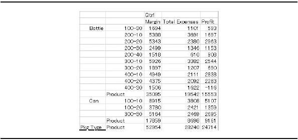
Figure 3-18. Pkg Type attribute dimension assigned to rows
You can use attribute dimensions in a report on any axis and navigate through them like any other dimension. In Figure 3-18, the Pkg Type attribute dimension is assigned to rows and is expanded to show its children: Bottle and Can.
If you zoom in on a level 0 attribute member, Essbase traverses the base dimension and brings back all members with an assigned attribute. For instance, in Figure 3-18, products 100-10, 100-20, and 300-30 are packaged in cans. The ability to navigate through the bottom of an attribute dimension and into the base dimension hierarchy is an advantage attribute dimensions have over shared members (pointers to existing members).
Another advantage of attribute dimensions is that you can assign them to a different axis than the base dimension (often called a cross-tab report) as shown in Figure 3-19.
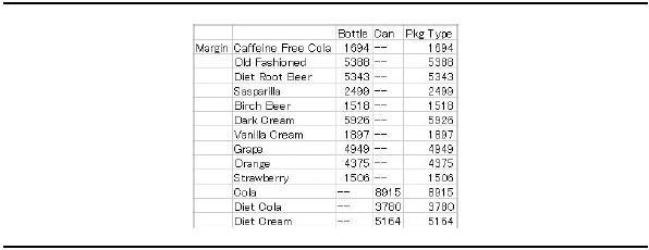
Figure 3-19. Attribute dimensions can be assigned to a different axis than the base dimension.
You can also take advantage of built-in calculations for attribute dimensions. By default, Essbase sums values for attribute dimensions dynamically (derived at query time, not stored). You can ask Essbase to derive the values in a variety of ways:
- Sum
- Count
- Min imum (Min)
- Maximum (Max)
- Average (Avg)
Sum is the default. To select a different representation, you enter the keyword (shown in parentheses in the preceding list) in the spreadsheet (see Figure 3-20). Note that you can enable alternate keywords as desired. This might be to match other languages or just to use preferred terms.
Because attribute values are derived dynamically, there are performance considerations when implementing alternate data views in this fashion.
Attributes can be of five types: text, date, Boolean, numeric, or linked value. The linked value attribute is a special attribute type reserved for Essbase. Linked value attributes are created automatically when building a date-time dimension type. They allow for the cross-tab reporting of time. Each time period is categorized by its characteristics in relationship to the other members in the time dimension. For example, a day might have an attribute that denotes that it is the third day of the week, twenty- third day of the month, and a Tuesday. The specific linked value attributes that are created are based on the selections you make when creating the date-time dimension.
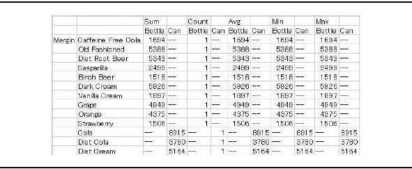
Figure 3-20. Built-in calculations for attribute dimensions are easy to use.
Depending on the attribute type, you can leverage the member's attribute values for further analysis. For example, if you wanted to derive profit per ounce, you could divide the total profit for a product SKU by its numeric ounces value. Essbase provides functions to let you query a member's attribute values.
Attribute dimensions are one way to provide alternate hierarchies. You can also use shared members to create an alternate hierarchy, or you can use user-defined attributes to group members differently.
In addition, any attribute association can be defined to vary across other dimensions. For example, the product manager for a product may vary across the additional dimensions of geography and time.
Essbase Data Types (Typed Measures)
Historically, Essbase was limited to storing only numbers. However, with more recent releases, Essbase has expanded its capabilities to store not only numeric data but also text and dates. From a design perspective, the capabilities that these data types provide either expand historical capabilities or serve to make specific types of analysis easier.
Numeric Measures The numeric data type is the default data type for Essbase. By default, all metrics are stored as doubles. Before version 11.x of Essbase, the numeric data type was the only storage format for data within an Essbase database.
Text Measures In Essbase, the text data type is associated with a text list. The text list takes a list of user-defined text tags that can be assigned to a measure or to any other member in any dimension. For example, you might have a metric to track customer satisfaction based on a scale from 1 to 3. Instead of showing the numerals 1,2, and 3 in a report, you can show High, Medium, and Low. Additionally, you can alter a value at a given intersection and use the write-back capabilities of Essbase to submit an updated satisfaction rating to the database.
Figure 3-21 shows how a text list looks in Smart View. In this tool, you can select text values from a drop-down list associated with a data cell. Regardless of the front- end reporting tool, Essbase provides the text tag so the reporting display is consistent.

Figure 3-21. In Oracle Hyperion Smart View for Office, text values are shown in a drop-down list for the selected data cell
Smart View is able to leverage some of the user interface capabilities of Microsoft Excel to provide additional functionality.
You can also do math across the text values. Internally, Essbase understands these strings as numbers. So, for example, you can take an average of customer satisfaction across a given region.
Thinking more about the database design, you might consider using text measures instead of attributes in some cases. For example, Figure 3-21 shows how a product is packaged in the data grid instead of using attributes as row or column headers. Leveraging text in this fashion lets you show how a product is packaged differently from region to region. Essentially, this accommodates the requirement of showing many-to-many relationships. When designing the analytical database, do not forget the reports. If there is a reporting requirement to show data (text included) in this fashion, then you should consider the use of textual data.
Date Measures Similar to text data, you can display date values in an Essbase report. This is done by specifying that a given member (generally a measure) is of type date. You can then specify the date format (MM-DD-YY, YYYY-DD-MM, and so on) for the output. Figure 3-22 shows an example of using a date type instead of, say, an attribute dimension for introduction date. Essbase understands the numeric value of the date, so you can easily perform date-differencing calculations (such as day's sales outstanding).
Alternate Views of the Data
In this article, we discussed how there is more than one way to look at data, and we introduced the general concepts of alternate hierarchies and user-defined attributes. In Essbase, you can create alternate hierarchies using shared members or attribute dimensions. You can also specify user-defined attributes. When designing your Essbase database, you need to make decisions about how to implement alternate
Figure 3-22. Sample report with date measures
views of the data. This section presents all three options, and then gives you some advice for choosing the most suitable option for your application.
Alternate Hierarchies Using Shared Members A shared member is a pointer to an existing member. This means that you can include a member in more than one dimension hierarchy while ensuring that the Essbase database does not store the member more than once. For example, Figure 3-23 shows an alternate hierarchy contained in the Sample Basic outline.
The Diet hierarchy contains a list of members representing the diet soda. We know the members are shared members because the tag Shared Member appears beside the member name. The actual members reside under Colas, Root Beer, and Cream Soda, respectively. The values of the shared members aggregate to the Diet member, thereby representing an alternate reporting structure and mathematical total within the Product dimension. Using this technique, you can minimize data storage (and disk space requirements), but still provide a broad range of reporting capabilities.
Alternate Hierarchies using Attribute Dimensions We discussed the attribute dimension approach to alternate hierarchies earlier, in the "Attribute Dimension and Base Dimension" section. Attribute dimensions have restrictions on when and how you can use them. Some of the restrictions are apparent in Table 3-1, which compares the alternate view methods. One restriction that is not obvious from the table is that attribute dimensions can be applied to only sparse dimensions in a block storage database. For more information about attributes and attribute dimensions, see the Oracle Essbase Database Administrator's Guide.

Figure 3-23. Alternate hierarchies can be created using shared members.

Figure 3-24. User-defined attributes are identified with the UDA tag.
User-Defined Attributes Recall that user-defined attributes are text tags that make it easier to find and display members in alternate ways. In Essbase, you can define as many tags as you need and associate those tags with members in any dimension and at any level. In the outline, members with attributes have an UDA tag followed by the attribute text, as shown in Figure 3-24.
When querying against an Essbase database, you can select members based on their user-defined attributes and bring them into the sheet. You use a member selector, such as that shown in Figure 3-25, to filter results by user-defined attributes.

Figure 3-25. User-defined attributes let you filter your results.
Unlike attribute dimensions, user-defined attributes do not provide any additional capabilities such as attribute calculations or cross-tab capabilities. They can, however, be assigned to any dimension, and a single member (such as New York, for the example in Figure 3-24) can have multiple user-defined attributes from the same category—neither of these apply with attribute dimensions. For example, if you have an attribute dimension for package type (bottles or cans), then you can assign a given product (such as Cola) the attribute of bottle or can, not both. Conversely, you could assign both if they were user-defined attributes.
Comparing Alternate View Methods It is almost inevitable that users will want to view data via multiple methods. You need to consider which technique to use to meet your users' needs. While there are no absolutes for choosing one method over another, Table 3-1 provides some guidance for making this choice.
Whichever way you choose to implement alternate views of the data, doing so means that you will be meeting a critical need of your end users to see and calculate data in a variety of ways.
Varying Attributes
Varying attributes can be thought of as an extension of the attribute capability. They are neither a dimension type nor a data type, but have elements of each to enable you to store data associations that change over other dimensions. Varying attributes let you vary information in one dimension by up to four additional dimensions. For example, if you classify employees by marital status or number of dependents, you can vary this over time. If an employee has no dependents in January, but has twins in April, you can classify data correctly in each time period.

Table 3-1. Comparison of Features Supported by the Alternate View Techniques

Figure 3-26. Varying attributes let you model slowly changing dimensions.
You can vary information across up to four independent dimensions. Using our package type attribute as an example, you could vary the packaging over time and geography, as shown in Figure 3-26.
There are no special client requirements to query a varying attribute. The structure is modeled into the database, and users simply query the information like any other Essbase data. However, using Smart View, it is possible to produce alternate views of the data based upon specific attribute associations, for example, view the data as it would have been if all associations were as specified in March.
Choosing a Data Storage Model
A key decision in design is the type of model you choose. When we talk about Essbase model types, we are not talking about the classifications of OLAP (MOLAP, HOLAP, ROLAP, and XOLAP). Rather, we are referring to the two storage types available within Essbase: aggregate storage and block storage.
Often, the model type is a direct result of user or analytic requirements. Other times, either Essbase model type can meet the requirements, and the choice is simply a matter of performance and maintenance considerations.
Block Storage
Block storage is the historical storage methodology in Essbase. Databases using this storage method hold data in small linear arrays, called blocks. The easiest way to think about a block storage model is by looking at a spreadsheet like the one in Figure 3-27. For the sake of this discussion, assume that the entire block structure is represented on this spreadsheet.
For every intersection where a piece of data exists, Essbase creates a block. Using our example, every block in the database contains all the members under Year and all of the members under Profit. Essbase also creates a block for every intersection of Product, Market, and the scenario (Actual, Budget, and so forth) where there is numeric data. For example, if you have a sale for product 100-10 in New York for the Actual scenario, one block is created. If you then put in a value in

Figure 3-27. Block storage saves data in blocks of memory.
for same product and market in the Budget scenario, a new block is created. And if you sell product 100-10 in Boston in the Actual scenario, this is another block.
All blocks have the same time periods and same accounts. The specific numeric values will most likely be different. Essbase preallocates the space for data storage. Whenever you query values from or submit values to the database, the specific block or blocks need to be brought into memory.
In general, block storage supports a smaller number of dimensions and overall members. For example, if there are 10,000 members in the Market dimension and 1,000 products, this represents 10,000,000 blocks (assuming every product has data for every market). But even though the overall dimensionality, members, and data tend to be smaller for block storage databases, these databases do not need to be small. We have worked with many block storage databases that have millions of members and hundreds of gigabytes of input data.
Block storage databases have the following functional advantages:
- Upper-level input You can input a total charge at an upper level, such as the dimension level, and then use an allocation method to push those values down to the members. For example, you can input a total charge at all markets and at all products and allocate the values down to individual product SKUs in individual cities. Upper-level inputs are particularly useful in situations where you want to do target budgeting or perform allocations such as a corporate overhead charge.
- Preaggregated values You can have Essbase precalculate every intersection. This means that query times (assuming the data request volume is synonymous) from request to request are consistent. In practice, however, many intersections of a block storage database are left to calculate dynamically at retrieval time. Total time period values, such as the total at Quarter 1, are often dynamically calculated as an overall efficiency practice
- Period-to-date reporting Period-to-date reporting capabilities come out of the box with block storage databases.
- Procedural calculations You have complete control over calculation behavior, down to the cellular level. If you need to model a complex calculation process, such as a goal-seeking calculation, you can control the process in detail with a calculation script.
Aggregate Storage
Aggregate storage databases store and manage data very differently from block storage databases. Instead of storing data in arrays (blocks), aggregate storage databases work with cells. In a block storage database, if you query a single value from a block, the entire structure comes into memory on the server. In an aggregate storage database, the same data that we used in the block storage example is represented as 136 data cells. Now if you query a single value, only that value is retrieved.
Because data structures are not preallocated, aggregate storage database can handle very expanded dimensionality and a lot more data. For instance, we have worked with models containing more than 10 million customers in a single dimension, as well as those with multiple millions of members per dimension in many dimensions.
With aggregate storage databases, data is loaded at level 0, and all upper-level members (for example, East) and member formulas are derived dynamically. To optimize retrieval performance, you can run an aggregation process on the database to build stored values at some upper-level intersections. After loading data, Essbase analyzes the source data and builds aggregates to optimize those queries that will take the longest to resolve based on the structure of the database. You can also have Essbase monitor the query patterns of your user base, and then build aggregations to serve your specific queries better. Essentially, the model is self-learning.
In general, aggregate storage models are ideal for aggregating large data sets (also called rack and stack applications). While you can do complex mathematics in aggregate storage models, all formulas are derived dynamically. A formula that is overly complex can affect performance. Although there are usually numerous ways to optimize processing in aggregate storage databases so that complex formulas do not have a large impact on performance, the dynamic nature of such formulas should be taken into consideration.
Aggregate storage databases provide the following advantages:
- Dimension, member, and data scale It is common to see aggregate storage databases with many millions members, with large dimensionality (20 or more dimensions), and being sourced with hundreds of gigabytes of data. In many cases, databases that could not be built in block storage work without difficulty in aggregate storage mode.
- Load and aggregation speed The smaller, cell-based structures tend to load more rapidly than blocks. Additionally, because you are not aggregating large portions of the database, but rather strategic points, the data is available to your users with less system downtime. Running an aggregation process, while recommended for performance reasons, is optional. Because all upper-level values are dynamic, the values at upper levels calculate on retrieval immediately after loading data.
- Smaller disk footprint Following the logic in the previous point, the overall structure of an aggregate storage database is smaller. A smaller structure coupled with a smaller aggregation footprint can lead to a disk footprint significantly smaller than that of a block storage database.
Selecting an Appropriate Data Storage Model
From an end-user perspective, querying an aggregate or block storage database is exactly the same. The nuances between the storage types are purely a deployment decision on the part of the Essbase database designer. At no point should an end user need to know how the data is handled within the database. Instead, you choose the model type based on the user requirements.
For example, we worked with a client who needed a six-dimensional model built with hundreds of gigabytes of input data. The company did not need any member formulas—the database was a series of simple aggregations and ratios. Our initial thought was to use aggregate storage. However, this company buys data, so the totals (for example, East) are not equal to the sum of the details (such as the children of East). In this case, we needed to load data at all levels in the database, which functionally is provided only by the block storage model. In addition, the company also had a ten-dimensional model that covered product SKU level information across 1.9 million customers. For this product database, we loaded level 0 data into an aggregate storage model. Your requirements may not always be so cut and dry. It is important to consider the attributes of each model type carefully, and especially the user requirements, before building the database.

table 3-2. Comparing Block and Aggregate Storage
Table 3-2 compares block storage and aggregate storage models based on user requirements. If both models can address the use requirement equally well, both columns are marked. If one is better at meeting the requirement, then it is selected, but this does not necessarily mean that the user requirement cannot be met by the other model (as shown by the example in the preceding paragraph, where we use block storage for a large input data set). For a list of current restrictions, see the Oracle Essbase Database Administrator's Guide.
Considering Partition Strategies
Previously, we talked about the importance of partitions in the data warehouse world, and mentioned how OLAP systems face some of the same challenges with respect to partitioning data. In Essbase, you can design applications with or without partitions, depending on the needs of your organization and the technical challenges of your environment.
Up until now, we have assumed that we are working with one Essbase database. As you will see, there are some very good reasons to implement multiple Essbase databases connected via partitions. To implement multiple databases, you need to create multiple Essbase applications. An Essbase application is essentially a container for an Essbase database and all the rules, reports, and metadata associated with that database. It is a best practice to have one database per application, though technically speaking, you could have more than one. Partitions allow you to manage and traverse data across multiple Essbase databases (and applications) seamlessly.
This section summarizes when you might want to partition data and outlines the types of partitions that are available. For more information, including guidelines, restrictions, and case studies, see the Oracle Essbase Database Administrator's Guide.
Reasons to Partition Data
You may want to partition your data for any of the following reasons:
- Differing dimensionality Different planning systems require different dimensionality. For example, you may want to budget costs for personnel, but that detail is unnecessary in a sales-focused application. You can create two applications and link them with a partition.
- Currency conversion This is a special case of differing dimensionality. Essbase has built-in features for creating a currency database and managing currency conversions.
- Redundancy You may want to have multiple copies of the same data available. For example, if your end users are reporting that they need to wait for access to a database, you can replicate the data to other databases and spread user access among the databases.
- Regional versions Remote offices may suffer from poor network response times, or they may need access when the master database is offline, so a local copy of the database is required.
- Local control over local data When a centrally administered database goes down, it affects everyone—local and remote. It may be preferable for remote offices to have control over their own data in local databases, with shared access to corporate data stored centrally.
- Security Not everyone needs to have access to all data. For example, personnel information is highly sensitive. This information can be safeguarded by maintaining the data separately and carefully controlling access to parts of the data via partitions. Although Essbase allows full security control within a database (to the individual cell level, if required), sometimes it can be easier to administer at the database level, or you may want different administrators for each database.
- Differing data storage Some data may be best stored in an aggregate storage database, while other data may be best handled in a block storage database. For example, an aggregate storage database can support writeback only to level 0. You might implement a block storage partition to handle changes to higher-level data for scenario playing or top-level adjustments. Additionally, you may wish to present a mix of stored data (aggregate storage or block storage), that is loaded daily, together with dynamic data from the data warehouse using an XOLAP database.
- Long timelines If you have (or plan to have) decades of data, you may want to store historical data separately, while retaining the ability to drill down into historical data from the current data.
- Regional batch windows If you have a composite database with data from multiple regions or business areas across different time zones, it may make sense to create different databases for each region and partition them together for presentation purposes.
Types of Partitions
Before we launch into a description of each of the partition types, let's start by defining some terminology. Figure 3-28 shows two multidimensional databases connected by a mapped partition. The source database is the primary database, which contains the stored multidimensional data. The target database is the secondary database—the one to which you copy or map stored data defined by a partition. Any given database can function as both a source database and a target database simultaneously. The partition area is the region of data to be shared.
A partition cell identifies the cell used in linked partitions.
Essbase offers three types of partitions: replicated, transparent, and linked. You can use different partition types within the same database, with some documented restrictions.
Replicated Partition With a replicated partition, Essbase copies data in the partition from the source database to the target database. The databases must share a similar dimensionality, and you need to map the dimensions, members, and attributes within the partition to the target database. As shown in Figure 3-29, a target database can be made up entirely from data copied from multiple source databases. For example, imagine that each of the source databases belong to a sales region. The summary data from each source database is partitioned and replicated to the target database, which is used by head office to analyze sales. The target database can also contain its own data, as well as additional data coming from other partitions.

Figure 3-28. Partition terminology

Figure 3-29. Replicated partitions copy data to another database.
The replicated data in the target database reflects the state of the data at the time the region was copied. The administrator updates partitions on a regular schedule, either by recopying the entire partition or by updating changed values. Periodic updates mean that at any given point in time, end users accessing the target database may be working with data that is not up-to-the-minute current. This may or may not be of concern. In many scenarios, such as analyzing past performance (for a month, quarter, or year for example), the data does not need to be up-to-date.
Transparent Partition If you do need up-to-the-minute data, a transparent partition may be more suitable. A transparent partition opens a window from the target database to the source database, as illustrated in Figure 3-30. End users can access data in the partition without the need to copy the data to the target database. As with replicated partitions, the source and target databases must share similar dimensionality, and you need to map the dimensions, members, and attributes in the partition to the target database.
End users query their target database as usual. Essbase retrieves data from the source database as required and presents it to the user as if it were part of the target database. If a user updates data that lives in the source database, the update is written back to the source database. Calculations may be faster because they are distributed across multiple databases (and potentially multiple computers and/or processors).

Figure 3-30. Transparent partitions connect databases.
While transparent partitions have clear advantages, they may also cause higher network traffic as Essbase retrieves data from the source database, which may be on a different server. If the number of retrievals becomes excessive, end users may experience slower response times. Implement transparent partitions using the documented guidelines to avoid this and other performance-related issues.
Linked Partition A linked partition is not so much a partition as a drill path associated with a data cell. As illustrated in Figure 3-31, the partition cell enables users to drill across from the target database to the source database. The target and source databases can have different dimensionality. The partition cell can be a single cell or a group of cells.
When an end user drills down on a partition cell in Excel, a new grid is created based on the data in the source database. Linked partitions are supported in Excel with Spreadsheet Add-in. Not all front-end reporting tools implement linked partition functionality, so check the documentation for any tools you use before implementing linked partitions. Finally, be sure to set user access separately for each database to ensure the security of the data. You do not want an end user linking to another database and having unrestricted access to potentially sensitive data.

Figure 3-31. Linked partitions enable drill-across to a database with different dimensionality.
Designing an OLAP Solution with Partitions
Partitions are the tools that can take you from a single, stand-alone database to a distributed Essbase solution tailored to meet your business needs and technical environment. When designing a distributed database model, you can use the following approaches:
- In a top-down approach, your primary database contains all your data, and the data is copied or mapped to other databases. For example, you could use this approach to create redundant or regional versions of a central database.
- A bottom-up approach takes data from a set of databases and presents that data together. Figure 3-29, which illustrates replicated partitions, shows a bottom-up approach: regional data is stored locally, and summary data goes to a target database at head office.
- For an attribute-driven approach, you create a partition that contains data for members that share the same user-defined attributes and map or copy that partition to a target database under a base dimension.
You can use the different partition types and strategies together to create a model that meets the unique needs of your organization. Bear in mind, however, that a distributed Essbase model adds layers of complexity to an OLAP solution. You need a solid understanding of each of the partition types and how they can be used together before beginning the design process.
Summary of the Essbase Design Process
Essbase is an independent OLAP solution that lets organizations extend their analytic and reporting in environments by providing large data scale, exemplary performance, and centralized control over metadata definitions and calculations. The driving factors in an Essbase deployment are the reporting requirements of the end user. While it is important to have a fundamental grounding in OLAP modeling, it is equally important to talk to the line-of-business users being served by the analytic system. In general, this drives most decisions, ranging from alternate hierarchy requirements, to data partitioning, to storage type.
After gaining the understanding of the overall reporting and analytics requirements, it is important to consider the built-in capabilities Essbase provides. Attribute dimensions, user-defined attributes, and shared members (for example) provide an array of capabilities without driving complex design or maintenance. In that same spirit, dimension types, built-in time-series calculations, and expense reporting capabilities can often serve to simplify the model and provide a greater level of user satisfaction. In short, do not forget to consider the out-of-box capabilities that Essbase provides.
In the my next blog, we look at the architecture of Oracle OLAP and Oracle Essbase and introduce the components for each product.